How to find Value with two or Multiple Criteria in Excel?

This article thoroughly describes the array formula and depicts the advanced filter to find the value with two or various constraints in excel. The criteria range for an Excel advanced filter is a collection of worksheet cells where the data filtering rules are entered. There must be a particular layout for the heading cells and criteria cells in the criteria range.

The vertical and horizontal lookup functions in Microsoft Excel are special functions, but experienced users typically replace them with INDEX MATCH, which is in many respects superior to VLOOKUP and HLOOKUP. It can search up two or more criteria in columns and rows, among other things.

Multiple Approaches

We have provided the solution using different approaches

• By using Array formula.

• By using advanced Filter

Approach 1: By using Array Formula

Here, a student record table as shown in image putting Array Formula 1 and excel can be used to find value using two or more parameters. By using the array formula, student grade value will be identified based one or more criteria.

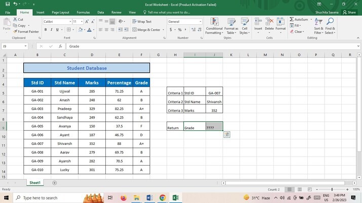
Step 1

The array formula for this problem is shown:

{=INDEX(array,MATCH(1,(criteria 1=lookup_array 1)*(criteria 2= lookup_array 2)…*(criteria n= lookup_array n),0))} 

Here, want to find the grade of Shivansh and Std_ID GA-007, can put array formula in cell J9, and after that simultaneously press the Ctrl + Shift + Enter keys.

=INDEX(F5:F14,MATCH(1,(J5=B5:B14)*(J6=C5:C14),0))

Note: The Grade column find value in is Cell F5:F14 in the calculation above. The Std ID and Std Name columns are Cell B5:B14 and Cell C5:C14, respectively. The very first criteria, Cell J5, is a Std ID, and the second requirement, Cell J6, is a Std Name.

Step 2

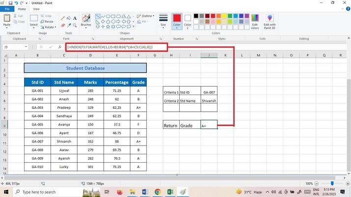
Formula for the array expression allows for the simple addition of parameters as necessary. If, for instance, you are searching for the Shivansh Grade where the Shivansh Marks is 352 and the Std ID is GA-007, include the following criteria as shown below:

=INDEX(F5:F14, MATCH(1,(J5=B5:B14)*(J6=C5:C14)*(J7=D5:D14),0))

Additionally, to obtain the Shivansh’s grade, press Ctrl + Shift + Enter simultaneously.

Step 3

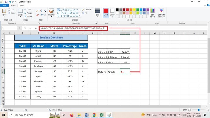
The following is the fundamental expression for this array formula:

=INDEX(array,MATCH(criteria1& criteria2…& criteriaN, lookup_array1& lookup_array2…& lookup_arrayN,0),0)

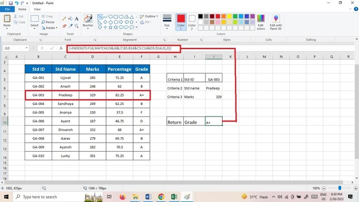
For illustration in the case, one can put the given formula into cell J9 and press Ctrl + Shift + Enter to determine the grade of Std whose Marks is 329 and Std ID is GA-003.

=INDEX(F5:F14,MATCH(J5&J6,B5:B14&D5:D14,0),0)

Note: The Grade column in the preceding formula is cell F5:F14. The Std ID column is B5:B14. The Marks column is cell D5:D14. Cell J5 is a Std ID as the first criterion, and cell J6 contains the Marks number that is specified as the second criterion.

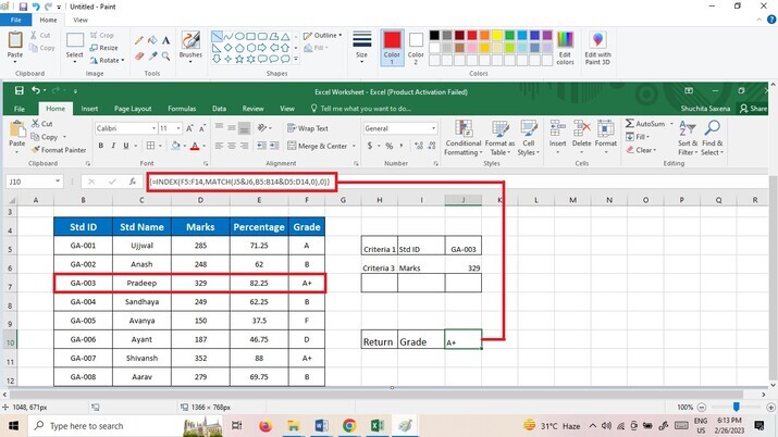
Step 4

If three or more factors were to be used to determine value, the criteria and lookup array can be easily added to the MATCH section. The lookup array and criteria must be in the same sequence, so please take note of this.

For example, we want to find out the grade of Pradeep with marks is 329 and Std Id is GA-003, the lookup array and parameters can be added as follows:

And sequentially press Ctrl+ Shift+ Enter.

=INDEX(F5:F14,MATCH(J5&J6&J7,B5:B14&C5:C14&D5:D14,0),0)

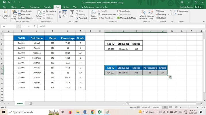
Approach 2: By using an Advanced Filter

To retrieve all values in Excel that meet two or more criteria regarding formulas, use the Advanced Filter feature. Do the following:

Step 1

Now click on Data menu and then go to the Advanced option under the Sort & Filter to turn on the Advanced Select feature.

Step 2

After opening the Advanced Filter dialog box, select the Copy to another location radio button in the Action Tab;

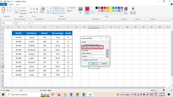
Step 3

Click on the List range box text box, choose the range cell B4:F14 to find values as shown below:

Step 4

Now click in the Criteria range box, find values by selecting the range I5:K6.

Step 5

By clicking Copy to box text box, the filtered rows will be placed in the destination range's first cell, I10.

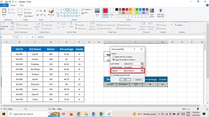
Step 6

Now click on OK button. If all the mentioned criteria are satisfied, the filtered rows are copied and put in the specified limit.

Conclusion

In this article, use simple example to show how to obtain value after applying more than two or more constraints in Excel. Users employ the multiplication operation, which serves as the array formulas AND operator, to assess multiple criteria. With the help of Advanced Filter, you can create a special list of things and extract them to another location in worksheet or workbook.