How to Exclude Values in One List from Another in Excel

Excel is a powerful tool that offers a variety of functions for data manipulation and analysis. Here we will first create a formula for excluding values in one list from another list in the Excel. Let us see the process that how we can achieve it.

These are the steps that need to be followed.

Step 1

Place your List 1 in one column and List 2 in another column. Let's assume List 1 is in column A, starting from cell A2, and List 2 is in column B, starting from cell B2.

Step 2

In cell C2 (adjacent to the first value in List 2), enter the following formula:

=IF(ISERROR(MATCH(B2, A:A, 0)), B2, "")

This formula uses the MATCH function to check if the value in cell B2 exists in List 1 (column A). If it doesn't find a match, it returns an error. The ISERROR function then checks if there is an error. If there is no match, it returns the value from List 2 (cell B2); otherwise, it returns an empty string.

Step 3

Copy the formula down to fill the rest of the cells in Column C. Excel will automatically adjust the cell references, so the formula references the correct rows for each cell.

Step 4

Column C will now display the values from List 2, excluding any values that exist in List 1.

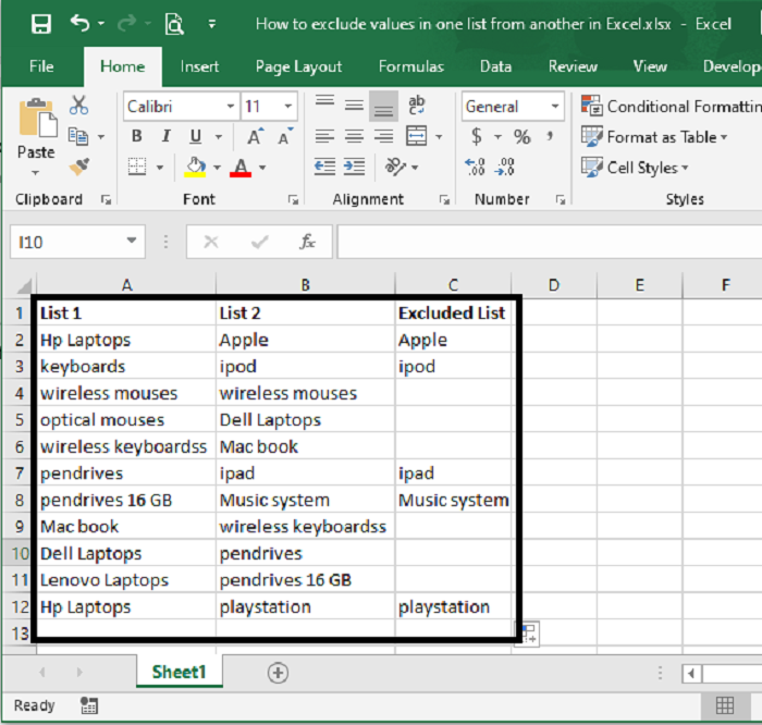
In the resulting Column C, the values from List 2 that are present in List 1 will be excluded, while the values that are not present in List 1 will remain.

Detailed Description of the Formula

The formula =IF(ISERROR(MATCH(B2, A:A, 0)), B2, "") consists of three main functions: ISERROR, MATCH, and IF. Let's break it down step by step:

MATCH Function: MATCH(B2, A:A, 0)

The MATCH function searches for a specified value (in this case, the value in cell B2) within a range (in this case, column A) and returns the relative position of that value within the range. The third argument, 0, indicates that an exact match is required.

If the value in cell B2 is found in column A, the MATCH function will return the relative position of that value in column A. If the value is not found, the MATCH function will return an error.

ISERROR Function: ISERROR(MATCH(B2, A:A, 0))

The ISERROR function checks if a given expression (in this case, the MATCH function) returns an error. It returns TRUE if there is an error, and FALSE if there is no error.

In the formula, we use ISERROR to check if the MATCH function returns an error. If there is an error, it means that the value in cell B2 was not found in column A.

IF Function: IF(ISERROR(MATCH(B2, A:A, 0)), B2, "")

The IF function evaluates a logical condition and returns one value if the condition is true, and another value if the condition is false.

In this formula, we use IF to check the result of the ISERROR function. If the ISERROR function returns TRUE (meaning there was an error in the MATCH function), it means that the value in cell B2 is not present in column A (List 1). In that case, we want to return the value from cell B2 itself (List 2). If the ISERROR function returns FALSE (meaning there was no error in the MATCH function), it means that the value in cell B2 is present in column A. In that case, we want to return an empty string ("").

Therefore, the final result of the IF function will be the value from cell B2 if it is not found in column A, and an empty string if it is found in column A.

By using this formula, you can compare the values in List 2 with List 1, and the resulting column will exclude any values that are present in List 1.

Conclusion

To exclude values from one list (List 1) that are present in another list (List 2) in Excel, you can use a combination of the MATCH, ISERROR, and IF functions. By comparing the values from List 2 against List 1, the formula identifies values that do not have a match in List 1 and excludes them. The resulting column displays the values from List 2 that are not found in List 1, making it convenient to analyze and compare data across different lists in Excel.