
Article Categories
- All Categories
-
 Data Structure
-
 Networking
-
 RDBMS
RDBMS
-
 Operating System
-
 Java
Java
-
 MS Excel
-
 iOS
iOS
-
 HTML
HTML
-
 CSS
CSS
-
 Android
-
 Python
-
 C Programming
-
 C++
C++
-
 C#
C#
-
 MongoDB
-
 MySQL
MySQL
-
 Javascript
-
 PHP
PHP
-
 Economics & Finance
How To Display The Corresponding Name Of The Highest Score In Excel?
Excel is a great tool for rapidly organising and analysing data. Finding the highest score in a dataset and extracting the name associated with that score is a typical task. This article will walk you through the step?by?step process of completing this work in Excel using formulae and functions. By the end of this article, you'll know exactly how to display the name of the individual who received the highest score in your Excel spreadsheet. So, let's get started and unleash the power of Excel to improve the effectiveness of your data analysis!
Display The Corresponding Name Of The Highest Score
Here, we will complete the task using a formula directly. So let us see a simple process to see how you can display the corresponding name of the highest score in Excel.
Step 1
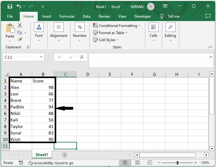
Consider an Excel sheet where the data in the sheet is similar to the below image.
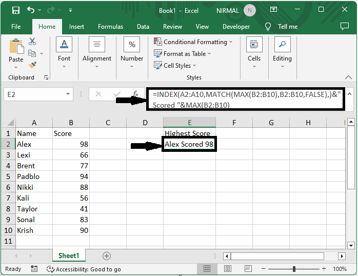
First, click on an empty cell and enter the formula as
=INDEX(A2:A10,MATCH(MAX(B2:B10),B2:B10,FALSE),)&" Scored "&MAX(B2:B10) and click enter to complete the task.
In the formula, A2:A10 is the range of cells containing names, and B2:B10 is the range of cells containing scores.
Empty cell > Formula > Enter.
This is how you can display the corresponding name of the highest score in Excel.
Note?
The formula will only display the name of the highest scorer, not multiple names. If your data has multiple users with the highest score, use the formula as
=INDEX($A$2:$A$10,SMALL(IF($B$2:$B$10=MAX($B$2:$B$10),ROW($B$2:$B$10)?1),ROW(B2)?1)) and click Ctrl + Shift + Enter, then drag using the autofill handle.
Conclusion
In this tutorial, we have used a simple example to demonstrate how you can display the corresponding name of the highest score in Excel to highlight a particular set of data.

8K+ Views
