- Signals & Systems Home
- Signals & Systems Overview
- Introduction
- Signals Basic Types
- Signals Classification
- Signals Basic Operations
- Systems Classification
- Types of Signals
- Representation of a Discrete Time Signal
- Continuous-Time Vs Discrete-Time Sinusoidal Signal
- Even and Odd Signals
- Properties of Even and Odd Signals
- Periodic and Aperiodic Signals
- Unit Step Signal
- Unit Ramp Signal
- Unit Parabolic Signal
- Energy Spectral Density
- Unit Impulse Signal
- Power Spectral Density
- Properties of Discrete Time Unit Impulse Signal
- Real and Complex Exponential Signals
- Addition and Subtraction of Signals
- Amplitude Scaling of Signals
- Multiplication of Signals
- Time Scaling of Signals
- Time Shifting Operation on Signals
- Time Reversal Operation on Signals
- Even and Odd Components of a Signal
- Energy and Power Signals
- Power of an Energy Signal over Infinite Time
- Energy of a Power Signal over Infinite Time
- Causal, Non-Causal, and Anti-Causal Signals
- Rectangular, Triangular, Signum, Sinc, and Gaussian Functions
- Signals Analysis
- Types of Systems
- What is a Linear System?
- Time Variant and Time-Invariant Systems
- Linear and Non-Linear Systems
- Static and Dynamic System
- Causal and Non-Causal System
- Stable and Unstable System
- Invertible and Non-Invertible Systems
- Linear Time-Invariant Systems
- Transfer Function of LTI System
- Properties of LTI Systems
- Response of LTI System
- Fourier Series
- Fourier Series
- Fourier Series Representation of Periodic Signals
- Fourier Series Types
- Trigonometric Fourier Series Coefficients
- Exponential Fourier Series Coefficients
- Complex Exponential Fourier Series
- Relation between Trigonometric & Exponential Fourier Series
- Fourier Series Properties
- Properties of Continuous-Time Fourier Series
- Time Differentiation and Integration Properties of Continuous-Time Fourier Series
- Time Shifting, Time Reversal, and Time Scaling Properties of Continuous-Time Fourier Series
- Linearity and Conjugation Property of Continuous-Time Fourier Series
- Multiplication or Modulation Property of Continuous-Time Fourier Series
- Convolution Property of Continuous-Time Fourier Series
- Convolution Property of Fourier Transform
- Parseval’s Theorem in Continuous Time Fourier Series
- Average Power Calculations of Periodic Functions Using Fourier Series
- GIBBS Phenomenon for Fourier Series
- Fourier Cosine Series
- Trigonometric Fourier Series
- Derivation of Fourier Transform from Fourier Series
- Difference between Fourier Series and Fourier Transform
- Wave Symmetry
- Even Symmetry
- Odd Symmetry
- Half Wave Symmetry
- Quarter Wave Symmetry
- Fourier Transform
- Fourier Transforms
- Fourier Transforms Properties
- Fourier Transform – Representation and Condition for Existence
- Properties of Continuous-Time Fourier Transform
- Table of Fourier Transform Pairs
- Linearity and Frequency Shifting Property of Fourier Transform
- Modulation Property of Fourier Transform
- Time-Shifting Property of Fourier Transform
- Time-Reversal Property of Fourier Transform
- Time Scaling Property of Fourier Transform
- Time Differentiation Property of Fourier Transform
- Time Integration Property of Fourier Transform
- Frequency Derivative Property of Fourier Transform
- Parseval’s Theorem & Parseval’s Identity of Fourier Transform
- Fourier Transform of Complex and Real Functions
- Fourier Transform of a Gaussian Signal
- Fourier Transform of a Triangular Pulse
- Fourier Transform of Rectangular Function
- Fourier Transform of Signum Function
- Fourier Transform of Unit Impulse Function
- Fourier Transform of Unit Step Function
- Fourier Transform of Single-Sided Real Exponential Functions
- Fourier Transform of Two-Sided Real Exponential Functions
- Fourier Transform of the Sine and Cosine Functions
- Fourier Transform of Periodic Signals
- Conjugation and Autocorrelation Property of Fourier Transform
- Duality Property of Fourier Transform
- Analysis of LTI System with Fourier Transform
- Relation between Discrete-Time Fourier Transform and Z Transform
- Convolution and Correlation
- Convolution in Signals and Systems
- Convolution and Correlation
- Correlation in Signals and Systems
- System Bandwidth vs Signal Bandwidth
- Time Convolution Theorem
- Frequency Convolution Theorem
- Energy Spectral Density and Autocorrelation Function
- Autocorrelation Function of a Signal
- Cross Correlation Function and its Properties
- Detection of Periodic Signals in the Presence of Noise (by Autocorrelation)
- Detection of Periodic Signals in the Presence of Noise (by Cross-Correlation)
- Autocorrelation Function and its Properties
- PSD and Autocorrelation Function
- Sampling
- Signals Sampling Theorem
- Nyquist Rate and Nyquist Interval
- Signals Sampling Techniques
- Effects of Undersampling (Aliasing) and Anti Aliasing Filter
- Different Types of Sampling Techniques
- Laplace Transform
- Laplace Transforms
- Common Laplace Transform Pairs
- Laplace Transform of Unit Impulse Function and Unit Step Function
- Laplace Transform of Sine and Cosine Functions
- Laplace Transform of Real Exponential and Complex Exponential Functions
- Laplace Transform of Ramp Function and Parabolic Function
- Laplace Transform of Damped Sine and Cosine Functions
- Laplace Transform of Damped Hyperbolic Sine and Cosine Functions
- Laplace Transform of Periodic Functions
- Laplace Transform of Rectifier Function
- Laplace Transforms Properties
- Linearity Property of Laplace Transform
- Time Shifting Property of Laplace Transform
- Time Scaling and Frequency Shifting Properties of Laplace Transform
- Time Differentiation Property of Laplace Transform
- Time Integration Property of Laplace Transform
- Time Convolution and Multiplication Properties of Laplace Transform
- Initial Value Theorem of Laplace Transform
- Final Value Theorem of Laplace Transform
- Parseval's Theorem for Laplace Transform
- Laplace Transform and Region of Convergence for right sided and left sided signals
- Laplace Transform and Region of Convergence of Two Sided and Finite Duration Signals
- Circuit Analysis with Laplace Transform
- Step Response and Impulse Response of Series RL Circuit using Laplace Transform
- Step Response and Impulse Response of Series RC Circuit using Laplace Transform
- Step Response of Series RLC Circuit using Laplace Transform
- Solving Differential Equations with Laplace Transform
- Difference between Laplace Transform and Fourier Transform
- Difference between Z Transform and Laplace Transform
- Relation between Laplace Transform and Z-Transform
- Relation between Laplace Transform and Fourier Transform
- Laplace Transform – Time Reversal, Conjugation, and Conjugate Symmetry Properties
- Laplace Transform – Differentiation in s Domain
- Laplace Transform – Conditions for Existence, Region of Convergence, Merits & Demerits
- Z Transform
- Z-Transforms (ZT)
- Common Z-Transform Pairs
- Z-Transform of Unit Impulse, Unit Step, and Unit Ramp Functions
- Z-Transform of Sine and Cosine Signals
- Z-Transform of Exponential Functions
- Z-Transforms Properties
- Properties of ROC of the Z-Transform
- Z-Transform and ROC of Finite Duration Sequences
- Conjugation and Accumulation Properties of Z-Transform
- Time Shifting Property of Z Transform
- Time Reversal Property of Z Transform
- Time Expansion Property of Z Transform
- Differentiation in z Domain Property of Z Transform
- Initial Value Theorem of Z-Transform
- Final Value Theorem of Z Transform
- Solution of Difference Equations Using Z Transform
- Long Division Method to Find Inverse Z Transform
- Partial Fraction Expansion Method for Inverse Z-Transform
- What is Inverse Z Transform?
- Inverse Z-Transform by Convolution Method
- Transform Analysis of LTI Systems using Z-Transform
- Convolution Property of Z Transform
- Correlation Property of Z Transform
- Multiplication by Exponential Sequence Property of Z Transform
- Multiplication Property of Z Transform
- Residue Method to Calculate Inverse Z Transform
- System Realization
- Cascade Form Realization of Continuous-Time Systems
- Direct Form-I Realization of Continuous-Time Systems
- Direct Form-II Realization of Continuous-Time Systems
- Parallel Form Realization of Continuous-Time Systems
- Causality and Paley Wiener Criterion for Physical Realization
- Discrete Fourier Transform
- Discrete-Time Fourier Transform
- Properties of Discrete Time Fourier Transform
- Linearity, Periodicity, and Symmetry Properties of Discrete-Time Fourier Transform
- Time Shifting and Frequency Shifting Properties of Discrete Time Fourier Transform
- Inverse Discrete-Time Fourier Transform
- Time Convolution and Frequency Convolution Properties of Discrete-Time Fourier Transform
- Differentiation in Frequency Domain Property of Discrete Time Fourier Transform
- Parseval’s Power Theorem
- Miscellaneous Concepts
- What is Mean Square Error?
- What is Fourier Spectrum?
- Region of Convergence
- Hilbert Transform
- Properties of Hilbert Transform
- Symmetric Impulse Response of Linear-Phase System
- Filter Characteristics of Linear Systems
- Characteristics of an Ideal Filter (LPF, HPF, BPF, and BRF)
- Zero Order Hold and its Transfer Function
- What is Ideal Reconstruction Filter?
- What is the Frequency Response of Discrete Time Systems?
- Basic Elements to Construct the Block Diagram of Continuous Time Systems
- BIBO Stability Criterion
- BIBO Stability of Discrete-Time Systems
- Distortion Less Transmission
- Distortionless Transmission through a System
- Rayleigh’s Energy Theorem
Fourier Transform of a Gaussian Signal
For a continuous-time function $\mathrm{x(t)}$, the Fourier transform of $\mathrm{x(t)}$ can be defined as,
$$\mathrm{X(\omega)\:=\:\int_{-\infty }^{\infty} x\left(t\right)\:e^{-j\omega t}\:dt}$$
Fourier Transform of Gaussian Signal
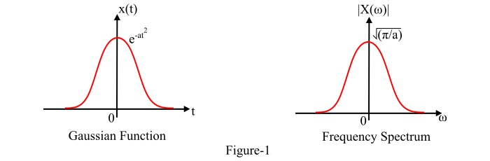
Gaussian Function - The Gaussian function is defined as,
$$\mathrm{g_{a}\left(t\right) \:=\: e^{-at^{2}} ;\:\:for\:all \:t}$$
Therefore, from the definition of Fourier transform, we have,
$$\mathrm{X(\omega) \:=\: F\left [e^{-at^2} \right ]\:=\:\int_{-\infty }^{\infty}e^{-at^2} \:e^{-j\omega t} \:dt}$$
$$\mathrm{\Rightarrow\: X\left(\omega\right) \:=\:\int_{-\infty}^{\infty} \:e^{-\left(at^2\:+\:j\omega t\right) }\:dt \:=\: e^{-\left(\omega^2/4a\right)}\int_{-\infty}^{\infty}\:e^{\left [{-t\sqrt{a}\:+\:(j\omega/2\sqrt{a})}\right]^{2}}dt }$$
Let,
$$\mathrm{\left [t\sqrt{a}\:+\:(j\omega 2\sqrt{a})\right ]\:=\: u}$$
Then,
$$\mathrm{du \:=\: \sqrt{a} \:dt\: and \: \:dt \:=\: \frac{du}{\sqrt{a}}}$$
$$\mathrm{\therefore\: X\left(\omega\right)\:=\:e^{-\left(\omega^2/4a\right)}\int_{-\infty }^{\infty}\: \frac{e^{-u^{2}}}{\sqrt{a}}\:du\: =\: \frac{e^{-\left(\omega^2/4a\right)}}{\sqrt{a}}\int_{-\infty }^{\infty}\:e^{-u^{2}} \:du}$$
$$\mathrm{\because\:\int_{-\infty }^{\infty}\:e^{-u^{2}} \:du \:=\: \sqrt{\pi}}$$
$$\mathrm{\therefore\: X\left(\omega\right) \:=\:\frac{e^{-\left(\omega^2/4a\right)}}{\sqrt{a}}\:\cdot\: \sqrt{\pi} \:=\: \sqrt{\frac{\pi}{a}} \:\cdot\: e^{-\left(\omega^2/4a\right)}}$$
Therefore, the Fourier transform of the Gaussian function is,
$$\mathrm{F\left [e^{-at^{2}}\right ] \:=\:\sqrt{\frac{\pi}{a}} \:\cdot\: e^{-\left ( \omega^2/4a\right )}}$$
Or, it can also be written as,
$$\mathrm{e^{-at^2}\overset{FT}{\leftrightarrow} \:\sqrt{\frac{\pi}{a}} \:\cdot\: e^{-\left (\omega^2/4a\right )}}$$
The graphical representation of Gaussian function and its frequency spectrum is shown in Figure-1.
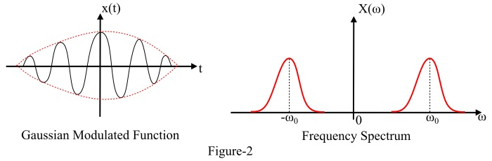
Fourier Transform of Gaussian Modulated Function
The Gaussian modulated signal is defined as
$$\mathrm{x\left(t \right) \:=\: e^{-at^{2}}\: cos \:\omega_{0}t}$$
$$\mathrm{\Rightarrow\: x\left(t \right)\ \:=\: e^{-at^{2}} \left (\frac{e^{j\omega_{0}t} \:+\: e^{-j\omega _{0}t}}{2}\right); \left\{\because\: cos \:\omega _{0}t \:=\:\left (\frac{e^{j\omega _{0}t} \:+\: e^{-j\omega_{0}t}}{2} \right) \right \}}$$
Therefore, the Fourier transform of the Gaussian modulated signal is
$$\mathrm{X\left( \omega\right) \:=\: \frac{1}{2} F\left [ e^{-at^{2}}e^{j\omega_{0}t} \right ] \:+\: \frac{1}{2}F\left [ e^{-at^{2}}e^{-j\omega _{0}t} \right ]}$$
By using frequency shifting property [i.e.$\mathrm{e^{-j\omega _{0}t}x\left (t\right)\overset{FT}{\leftrightarrow}X \left(\omega \:+\: \omega_{0}\right)}$] of Fourier transform, we get,
$$\mathrm{F\left[e^{-at^{2}}e^{j\omega _{0}t} \right] \:=\: F\left [e^{-at^{2}} \right]|_{\omega \:=\: \left ( \omega\:-\:\omega _{0}\right )}}$$
And
$$\mathrm{F\left[e^{-at^{2}}e^{-j\omega _{0}t} \right] \:=\:F\left [e^{-at^{2}} \right]|_{\omega \:=\: \left ( \omega \:+\: \omega _{0}\right )}}$$
Also, the Fourier transform of Gaussian function is,
$$\mathrm{F\left [e^{-at^{2}}\right ] \:=\: \sqrt{\frac{\pi}{a}} \cdot e^{-\left ( \omega^2/4a\right )}}$$
Therefore, the Fourier transform of Gaussian modulated function is,
$$\mathrm{X\left( \omega\right) \:=\: \frac{1}{2}\left[\sqrt{\frac{\pi}{a}} \:\cdot\: e^{-\left [\left(\omega\:-\:\omega _{0}\right)^{2}/4a\right]} \:+\: \sqrt{\frac{\pi}{a}} \:\cdot\: e^{-\left [\left(\omega \:+\: \omega _{0}\right)^{2}/4a\right ] } \right ]}$$
Or, it can also be represented as,
$$\mathrm{e^{-at^{2}}\: cos \:\omega _{0}t\overset{FT}{\leftrightarrow}\frac{1}{2}\left[\sqrt{\frac{\pi}{a}} \:\cdot\: e^{-\left [\left(\omega \:-\:\omega _{0}\right)^{2}/4a\right]} \:+\: \sqrt{\frac{\pi}{a}} \:\cdot\: e^{-\left [\left(\omega \:+\: \omega _{0}\right)^{2}/4a\right]}\right ]}$$
The graphical representation of the Gaussian modulated signal and its frequency spectrum is shown in Figure-2.