Article Categories
- All Categories
-
 Data Structure
-
 Networking
-
 RDBMS
RDBMS
-
 Operating System
-
 Java
Java
-
 MS Excel
-
 iOS
iOS
-
 HTML
HTML
-
 CSS
CSS
-
 Android
-
 Python
-
 C Programming
-
 C++
C++
-
 C#
C#
-
 MongoDB
-
 MySQL
MySQL
-
 Javascript
-
 PHP
PHP
-
 Economics & Finance
Fast Fourier Transform (FFT) on Arduino
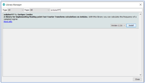
There are several libraries available which help you calculate the Fast Fourier Transform (FFT) onboard the Arduino. We will look at the arduinoFFT library. This library can be installed via the Library Manager (search for arduinoFFT).

Once installed, go to: File→Examples→arduinoFFT and open the FFT_01 example.
Example
This example first creates a sinusoidal wave with the frequency of 1000Hz (sampled at 5000Hz). It then windows this using a Hamming function. Later it computes the FFT, determines the frequency with the highest magnitude, and returns it as the fundamental frequency. If that value is close to 1000 Hz, this code works.
Let's begin the code walkthrough. We first include the library and create the arduinoFFT() object.
#include "arduinoFFT.h"

arduinoFFT FFT = arduinoFFT(); // Create FFT object
We then define the variables specific to the signal.
const uint16_t samples = 64; //This value MUST ALWAYS be a power of 2
const double signalFrequency = 1000;
const double samplingFrequency = 5000;
const uint8_t amplitude = 100;
We will use 64 samples of the signal to generate our time domain array. Also, this number of sample should always be a power of 2.
Later, we define two arrays to store the Real and Imaginary parts of the FFT output finally, and the raw data initially.
double vReal[samples];
double vImag[samples];
Finally, 4 constants are defined. These are passed on as arguments in the printVector() function that is defined later, and help determine the scaling factor. We'll see their usage when we walk through the printVector() function.
#define SCL_INDEX 0x00
#define SCL_TIME 0x01
#define SCL_FREQUENCY 0x02
#define SCL_PLOT 0x03
Within the setup, we simply initialize Serial.
void setup()
{
   Serial.begin(115200);
   while(!Serial);
   Serial.println("Ready");
}
In the loop, we first construct our time-domain signal array.
void loop()
{
   /* Build raw data */

   // Number of signal cycles that the sampling will read
   double cycles = (((samples-1) * signalFrequency) / samplingFrequency);
   for (uint16_t i = 0; i < samples; i++)
   {
   /* Build data with positive and negative values*/
   vReal[i] = int8_t((amplitude * (sin((i * (twoPi * cycles)) / samples))) / 2.0);
   // vReal[i] = uint8_t((amplitude * (sin((i * (twoPi * cycles)) / samples) + 1.0)) / 2.0);
   /* Build data displaced on the Y axis to include only positive values*/
   /* Imaginary part must be zeroed in case of looping to avoid wrong calculations and overflows */
   vImag[i] = 0.0;
   }
We then print the signal, apply the hamming window on the signal and print it again. We then compute the FFT, using FFT.Compute(), and print the real and imaginary vectors. Later we compute the magnitude from the real and imaginary vectors, using FFT.ComplexToMagnitude(), and print the magnitude.
Finally, we compute the frequency with the highest magnitude (using FFT.majorPeak()) and print it.
On running this, the frequency with the highest magnitude turns out to be 1004.225670, which is quite close to 1000 Hz.
/* Print the results of the simulated sampling according to time */
   Serial.println("Data:");
   PrintVector(vReal, samples, SCL_TIME);

   /* Weigh data */
   FFT.Windowing(vReal, samples, FFT_WIN_TYP_HAMMING, FFT_FORWARD);
   Serial.println("Weighed data:");
   PrintVector(vReal, samples, SCL_TIME);
   FFT.Compute(vReal, vImag, samples, FFT_FORWARD); //Compute FFT
   Serial.println("Computed Real values:");
   PrintVector(vReal, samples, SCL_INDEX);
   Serial.println("Computed Imaginary values:");
   PrintVector(vImag, samples, SCL_INDEX);
   FFT.ComplexToMagnitude(vReal, vImag, samples); // Compute magnitudes
   Serial.println("Computed magnitudes:");
   PrintVector(vReal, (samples >> 1), SCL_FREQUENCY);
   double x = FFT.MajorPeak(vReal, samples, samplingFrequency);
   Serial.println(x, 6);
   while(1);          / * Run Once */
   // delay(2000);    /* Repeat after delay */
}
Finally, the printVector function is defined.
This function takes in the vector to be printed, the number of entries to be printed, and the scaling factor.
If the factor is SCL_INDEX, the index number of each entry in the vector is printed.
If the factor is SCL_TIME, the time for each entry in the vector is printed starting from 0 (using sampling frequency). If the sampling frequency is 100, it takes 1/100 or 0.01 seconds for each reading. Thus, the time can be calculated for each reading.
If the factor is SCL_FREQUENCY, the frequency corresponding to each entry is printed. Note that this is only used after the magnitudes have been computed.
PrintVector(vReal, (samples >> 1), SCL_FREQUENCY);
Note that we have right shifted samples by 1. Since samples are always a power of 2, right shift would mean dividing number of samples by 2. Thus, for 64 samples, the value after right shift by 1 becomes 32.
The FFT gives frequency values from 0 to sampling frequency/2 (Nyquist criteria). Thus, the value of the frequency at each index is index*sampling_frequency/n_samples. This is how we get the frequencies.
void PrintVector(double *vData, uint16_t bufferSize, uint8_t scaleType)
{
   for (uint16_t i = 0; i < bufferSize; i++)
   {
      double abscissa;
      /* Print abscissa value */
      switch (scaleType)
      {
         case SCL_INDEX:
         abscissa = (i * 1.0);
      break;
      case SCL_TIME:
         abscissa = ((i * 1.0) / samplingFrequency);
      break;
      case SCL_FREQUENCY:
         abscissa = ((i * 1.0 * samplingFrequency) / samples);
      break;
   }
   Serial.print(abscissa, 6);
   if(scaleType==SCL_FREQUENCY)
      Serial.print("Hz");
      Serial.print(" ");
      Serial.println(vData[i], 4);
   }
   Serial.println();
}
Note that the relation between the computed magnitude and the amplitude of the original signal has not yet been established. You are encouraged to go through the other examples that come along with this library.


