- Elasticsearch - Home
- Elasticsearch - Basic Concepts
- Elasticsearch - Installation
- Elasticsearch - Populate
- Migration between Versions
- Elasticsearch - API Conventions
- Elasticsearch - Document APIs
- Elasticsearch - Search APIs
- Elasticsearch - Aggregations
- Elasticsearch - Index APIs
- Elasticsearch - CAT APIs
- Elasticsearch - Cluster APIs
- Elasticsearch - Query DSL
- Elasticsearch - Mapping
- Elasticsearch - Analysis
- Elasticsearch - Modules
- Elasticsearch - Index Modules
- Elasticsearch - Ingest Node
- Elasticsearch - Managing Index Lifecycle
- Elasticsearch - SQL Access
- Elasticsearch - Monitoring
- Elasticsearch - Rollup Data
- Elasticsearch - Frozen Indices
- Elasticsearch - Testing
- Elasticsearch - Kibana Dashboard
- Elasticsearch - Filtering by Field
- Elasticsearch - Data Tables
- Elasticsearch - Region Maps
- Elasticsearch - Pie Charts
- Elasticsearch - Area and Bar Charts
- Elasticsearch - Time Series
- Elasticsearch - Tag Clouds
- Elasticsearch - Heat Maps
- Elasticsearch - Canvas
- Elasticsearch - Logs UI
- Elasticsearch Useful Resources
- Elasticsearch - Quick Guide
- Elasticsearch - Useful Resources
- Elasticsearch - Discussion
Elasticsearch - Quick Guide
Elasticsearch - Basic Concepts
Elasticsearch is an Apache Lucene-based search server. It was developed by Shay Banon and published in 2010. It is now maintained by Elasticsearch BV. Its latest version is 7.0.0.
Elasticsearch is a real-time distributed and open source full-text search and analytics engine. It is accessible from RESTful web service interface and uses schema less JSON (JavaScript Object Notation) documents to store data. It is built on Java programming language and hence Elasticsearch can run on different platforms. It enables users to explore very large amount of data at very high speed.
General Features
The general features of Elasticsearch are as follows −
Elasticsearch is scalable up to petabytes of structured and unstructured data.
Elasticsearch can be used as a replacement of document stores like MongoDB and RavenDB.
Elasticsearch uses denormalization to improve the search performance.
Elasticsearch is one of the popular enterprise search engines, and is currently being used by many big organizations like Wikipedia, The Guardian, StackOverflow, GitHub etc.
Elasticsearch is an open source and available under the Apache license version 2.0.
Key Concepts
The key concepts of Elasticsearch are as follows −
Node
It refers to a single running instance of Elasticsearch. Single physical and virtual server accommodates multiple nodes depending upon the capabilities of their physical resources like RAM, storage and processing power.
Cluster
It is a collection of one or more nodes. Cluster provides collective indexing and search capabilities across all the nodes for entire data.
Index
It is a collection of different type of documents and their properties. Index also uses the concept of shards to improve the performance. For example, a set of document contains data of a social networking application.
Document
It is a collection of fields in a specific manner defined in JSON format. Every document belongs to a type and resides inside an index. Every document is associated with a unique identifier called the UID.
Shard
Indexes are horizontally subdivided into shards. This means each shard contains all the properties of document but contains less number of JSON objects than index. The horizontal separation makes shard an independent node, which can be store in any node. Primary shard is the original horizontal part of an index and then these primary shards are replicated into replica shards.
Replicas
Elasticsearch allows a user to create replicas of their indexes and shards. Replication not only helps in increasing the availability of data in case of failure, but also improves the performance of searching by carrying out a parallel search operation in these replicas.
Advantages
Elasticsearch is developed on Java, which makes it compatible on almost every platform.
Elasticsearch is real time, in other words after one second the added document is searchable in this engine
Elasticsearch is distributed, which makes it easy to scale and integrate in any big organization.
Creating full backups are easy by using the concept of gateway, which is present in Elasticsearch.
Handling multi-tenancy is very easy in Elasticsearch when compared to Apache Solr.
Elasticsearch uses JSON objects as responses, which makes it possible to invoke the Elasticsearch server with a large number of different programming languages.
Elasticsearch supports almost every document type except those that do not support text rendering.
Disadvantages
Elasticsearch does not have multi-language support in terms of handling request and response data (only possible in JSON) unlike in Apache Solr, where it is possible in CSV, XML and JSON formats.
Occasionally, Elasticsearch has a problem of Split brain situations.
Comparison between Elasticsearch and RDBMS
In Elasticsearch, index is similar to tables in RDBMS (Relation Database Management System). Every table is a collection of rows just as every index is a collection of documents in Elasticsearch.
The following table gives a direct comparison between these terms−
| Elasticsearch | RDBMS |
|---|---|
| Cluster | Database |
| Shard | Shard |
| Index | Table |
| Field | Column |
| Document | Row |
Elasticsearch - Installation
In this chapter, we will understand the installation procedure of Elasticsearch in detail.
To install Elasticsearch on your local computer, you will have to follow the steps given below −
Step 1 − Check the version of java installed on your computer. It should be java 7 or higher. You can check by doing the following −
In Windows Operating System (OS) (using command prompt)−
> java -version
In UNIX OS (Using Terminal) −
$ echo $JAVA_HOME
Step 2 − Depending on your operating system, download Elasticsearch from www.elastic.co as mentioned below −
For windows OS, download ZIP file.
For UNIX OS, download TAR file.
For Debian OS, download DEB file.
For Red Hat and other Linux distributions, download RPN file.
APT and Yum utilities can also be used to install Elasticsearch in many Linux distributions.
Step 3 − Installation process for Elasticsearch is simple and is described below for different OS −
Windows OS− Unzip the zip package and the Elasticsearch is installed.
UNIX OS− Extract tar file in any location and the Elasticsearch is installed.
$wget
https://artifacts.elastic.co/downloads/elasticsearch/elasticsearch7.0.0-linux-x86_64.tar.gz

$tar -xzf elasticsearch-7.0.0-linux-x86_64.tar.gz
Using APT utility for Linux OS− Download and install the Public Signing Key
$ wget -qo - https://artifacts.elastic.co/GPG-KEY-elasticsearch | sudo
apt-key add -
Save the repository definition as shown below −
$ echo "deb https://artifacts.elastic.co/packages/7.x/apt stable main" |
sudo tee -a /etc/apt/sources.list.d/elastic-7.x.list
Run update using the following command −
$ sudo apt-get update
Now you can install by using the following command −
$ sudo apt-get install elasticsearch
Download and install the Debian package manually using the command given here −
$wget https://artifacts.elastic.co/downloads/elasticsearch/elasticsearch7.0.0-amd64.deb
$sudo dpkg -i elasticsearch-7.0.0-amd64.deb0
Using YUM utility for Debian Linux OS
Download and install the Public Signing Key −
$ rpm --import https://artifacts.elastic.co/GPG-KEY-elasticsearch
ADD the following text in the file with .repo suffix in your /etc/yum.repos.d/ directory. For example, elasticsearch.repo
elasticsearch-7.x]
name=Elasticsearch repository for 7.x packages
baseurl=https://artifacts.elastic.co/packages/7.x/yum
gpgcheck=1
gpgkey=https://artifacts.elastic.co/GPG-KEY-elasticsearch
enabled=1
autorefresh=1
type=rpm-md
You can now install Elasticsearch by using the following command
sudo yum install elasticsearch
Step 4 − Go to the Elasticsearch home directory and inside the bin folder. Run the elasticsearch.bat file in case of Windows or you can do the same using command prompt and through terminal in case of UNIX rum Elasticsearch file.
In Windows
> cd elasticsearch-2.1.0/bin
> elasticsearch
In Linux
$ cd elasticsearch-2.1.0/bin
$ ./elasticsearch
Note − In case of windows, you might get an error stating JAVA_HOME is not set, please set it in environment variables to C:\Program Files\Java\jre1.8.0_31 or the location where you installed java.
Step 5 − The default port for Elasticsearch web interface is 9200 or you can change it by changing http.port inside the elasticsearch.yml file present in bin directory. You can check if the server is up and running by browsing http://localhost:9200. It will return a JSON object, which contains the information about the installed Elasticsearch in the following manner −
{
   "name" : "Brain-Child",
   "cluster_name" : "elasticsearch", "version" : {
      "number" : "2.1.0",
      "build_hash" : "72cd1f1a3eee09505e036106146dc1949dc5dc87",
      "build_timestamp" : "2015-11-18T22:40:03Z",
      "build_snapshot" : false,
      "lucene_version" : "5.3.1"
   },
   "tagline" : "You Know, for Search"
}
Step 6 − In this step, let us install Kibana. Follow the respective code given below for installing on Linux and Windows −
For Installation on Linux −
wget https://artifacts.elastic.co/downloads/kibana/kibana-7.0.0-linuxx86_64.tar.gz

tar -xzf kibana-7.0.0-linux-x86_64.tar.gz

cd kibana-7.0.0-linux-x86_64/

./bin/kibana
For Installation on Windows −
Download Kibana for Windows from https://www.elastic.co/downloads/kibana Once you click the link, you will find the home page as shown below −
Unzip and go to the Kibana home directory and then run it.
CD c:\kibana-7.0.0-windows-x86_64
.\bin\kibana.bat
Elasticsearch - Populate
In this chapter, let us learn how to add some index, mapping and data to Elasticsearch. Note that some of this data will be used in the examples explained in this tutorial.
Create Index
You can use the following command to create an index −
PUT school
Response
If the index is created, you can see the following output −
{"acknowledged": true}
Add data
Elasticsearch will store the documents we add to the index as shown in the following code. The documents are given some IDs which are used in identifying the document.
Request Body
POST school/_doc/10
{
   "name":"Saint Paul School", "description":"ICSE Afiliation",
   "street":"Dawarka", "city":"Delhi", "state":"Delhi", "zip":"110075",
   "location":[28.5733056, 77.0122136], "fees":5000,
   "tags":["Good Faculty", "Great Sports"], "rating":"4.5"
}
Response
{
   "_index" : "school",
   "_type" : "_doc",
   "_id" : "10",
   "_version" : 1,
   "result" : "created",
   "_shards" : {
      "total" : 2,
      "successful" : 1,
      "failed" : 0
   },
   "_seq_no" : 2,
   "_primary_term" : 1
}
Here, we are adding another similar document.
POST school/_doc/16
{
   "name":"Crescent School", "description":"State Board Affiliation",
   "street":"Tonk Road",
   "city":"Jaipur", "state":"RJ", "zip":"176114","location":[26.8535922,75.7923988],
   "fees":2500, "tags":["Well equipped labs"], "rating":"4.5"
}
Response
{
   "_index" : "school",
   "_type" : "_doc",
   "_id" : "16",
   "_version" : 1,
   "result" : "created",
   "_shards" : {
      "total" : 2,
      "successful" : 1,
      "failed" : 0
   },
   "_seq_no" : 9,
   "_primary_term" : 7
}
In this way, we will keep adding any example data that we need for our working in the upcoming chapters.
Adding Sample Data in Kibana
Kibana is a GUI driven tool for accessing the data and creating the visualization. In this section, let us understand how we can add sample data to it.
In the Kibana home page, choose the following option to add sample ecommerce data −
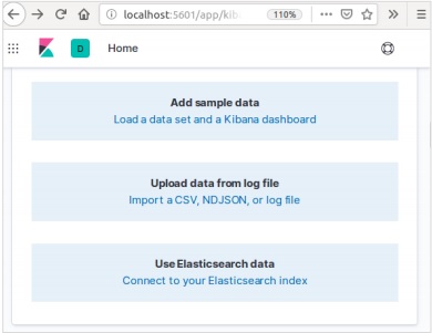
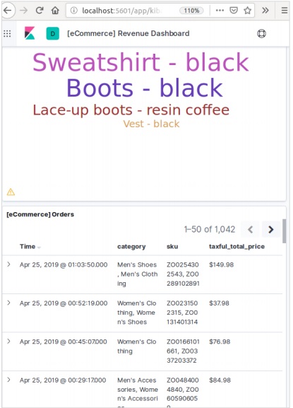
The next screen will show some visualization and a button to Add data −

Clicking on Add Data will show the following screen which confirms the data has been added to an index named eCommerce.
Elasticsearch - Migration between Versions
In any system or software, when we are upgrading to newer version, we need to follow a few steps to maintain the application settings, configurations, data and other things. These steps are required to make the application stable in new system or to maintain the integrity of data (prevent data from getting corrupt).
You need to follow the following steps to upgrade Elasticsearch −
Read Upgrade docs from https://www.elastic.co/
Test the upgraded version in your non production environments like in UAT, E2E, SIT or DEV environment.
Note that rollback to previous Elasticsearch version is not possible without data backup. Hence, a data backup is recommended before upgrading to a higher version.
We can upgrade using full cluster restart or rolling upgrade. Rolling upgrade is for new versions. Note that there is no service outage, when you are using rolling upgrade method for migration.
Steps for Upgrade
Test the upgrade in a dev environment before upgrading your production cluster.
Back up your data. You cannot roll back to an earlier version unless you have a snapshot of your data.
Consider closing machine learning jobs before you start the upgrade process. While machine learning jobs can continue to run during a rolling upgrade, it increases the overhead on the cluster during the upgrade process.
Upgrade the components of your Elastic Stack in the following order −
- Elasticsearch
- Kibana
- Logstash
- Beats
- APM Server
Upgrading from 6.6 or Earlier
To upgrade directly to Elasticsearch 7.1.0 from versions 6.0-6.6, you must manually reindex any 5.x indices you need to carry forward, and perform a full cluster restart.
Full Cluster Restart
The process of full cluster restart involves shutting down each node in the cluster, upgrading each node to 7x and then restarting the cluster.
Following are the high level steps that need to be carried out for full cluster restart −
- Disable shard allocation
- Stop indexing and perform a synced flush
- Shutdown all nodes
- Upgrade all nodes
- Upgrade any plugins
- Start each upgraded node
- Wait for all nodes to join the cluster and report a status of yellow
- Re-enable allocation
Once allocation is re-enabled, the cluster starts allocating the replica shards to the data nodes. At this point, it is safe to resume indexing and searching, but your cluster will recover more quickly if you can wait until all primary and replica shards have been successfully allocated and the status of all nodes is green.
Elasticsearch - API Conventions
Application Programming Interface (API) in web is a group of function calls or other programming instructions to access the software component in that particular web application. For example, Facebook API helps a developer to create applications by accessing data or other functionalities from Facebook; it can be date of birth or status update.
Elasticsearch provides a REST API, which is accessed by JSON over HTTP. Elasticsearch uses some conventions which we shall discuss now.
Multiple Indices
Most of the operations, mainly searching and other operations, in APIs are for one or more than one indices. This helps the user to search in multiple places or all the available data by just executing a query once. Many different notations are used to perform operations in multiple indices. We will discuss a few of them here in this chapter.
Comma Separated Notation
POST /index1,index2,index3/_search
Request Body
{
   "query":{
      "query_string":{
         "query":"any_string"
      }
   }
}
Response
JSON objects from index1, index2, index3 having any_string in it.
_all Keyword for All Indices
POST /_all/_search
Request Body
{
   "query":{
      "query_string":{
         "query":"any_string"
      }
   }
}
Response
JSON objects from all indices and having any_string in it.
Wildcards ( * , + , )
POST /school*/_search
Request Body
{
   "query":{
      "query_string":{
         "query":"CBSE"
      }
   }
}
Response
JSON objects from all indices which start with school having CBSE in it.
Alternatively, you can use the following code as well −
POST /school*,-schools_gov /_search
Request Body
{
   "query":{
      "query_string":{
         "query":"CBSE"
      }
   }
}
Response
JSON objects from all indices which start with school but not from schools_gov and having CBSE in it.
There are also some URL query string parameters −
- ignore_unavailable − No error will occur or no operation will be stopped, if the one or more index(es) present in the URL does not exist. For example, schools index exists, but book_shops does not exist.
POST /school*,book_shops/_search
Request Body
{
   "query":{
      "query_string":{
         "query":"CBSE"
      }
   }
}
Request Body
{
   "error":{
      "root_cause":[{
         "type":"index_not_found_exception", "reason":"no such index",
         "resource.type":"index_or_alias", "resource.id":"book_shops",
         "index":"book_shops"
      }],
      "type":"index_not_found_exception", "reason":"no such index",
      "resource.type":"index_or_alias", "resource.id":"book_shops",
      "index":"book_shops"
   },"status":404
}
Consider the following code −
POST /school*,book_shops/_search?ignore_unavailable = true
Request Body
{
   "query":{
      "query_string":{
         "query":"CBSE"
      }
   }
}
Response (no error)
JSON objects from all indices which start with school having CBSE in it.
allow_no_indices
true value of this parameter will prevent error, if a URL with wildcard results in no indices. For example, there is no index that starts with schools_pri −
POST /schools_pri*/_search?allow_no_indices = true
Request Body
{
   "query":{
      "match_all":{}
   }
}
Response (No errors)
{
   "took":1,"timed_out": false, "_shards":{"total":0, "successful":0, "failed":0},
   "hits":{"total":0, "max_score":0.0, "hits":[]}
}
expand_wildcards
This parameter decides whether the wildcards need to be expanded to open indices or closed indices or perform both. The value of this parameter can be open and closed or none and all.
For example, close index schools −
POST /schools/_close
Response
{"acknowledged":true}
Consider the following code −
POST /school*/_search?expand_wildcards = closed
Request Body
{
   "query":{
      "match_all":{}
   }
}
Response
{
   "error":{
      "root_cause":[{
         "type":"index_closed_exception", "reason":"closed", "index":"schools"
      }],
      "type":"index_closed_exception", "reason":"closed", "index":"schools"
   }, "status":403
}
Date Math Support in Index Names
Elasticsearch offers a functionality to search indices according to date and time. We need to specify date and time in a specific format. For example, accountdetail-2015.12.30, index will store the bank account details of 30th December 2015. Mathematical operations can be performed to get details for a particular date or a range of date and time.
Format for date math index name −
<static_name{date_math_expr{date_format|time_zone}}>
/<accountdetail-{now-2d{YYYY.MM.dd|utc}}>/_search
static_name is a part of expression which remains the same in every date math index like account detail. date_math_expr contains the mathematical expression that determines the date and time dynamically like now-2d. date_format contains the format in which the date is written in index like YYYY.MM.dd. If todays date is 30th December 2015, then <accountdetail-{now-2d{YYYY.MM.dd}}> will return accountdetail-2015.12.28.
| Expression | Resolves to |
|---|---|
| <accountdetail-{now-d}> | accountdetail-2015.12.29 |
| <accountdetail-{now-M}> | accountdetail-2015.11.30 |
| <accountdetail-{now{YYYY.MM}}> | accountdetail-2015.12 |
We will now see some of the common options available in Elasticsearch that can be used to get the response in a specified format.
Pretty Results
We can get response in a well-formatted JSON object by just appending a URL query parameter, i.e., pretty = true.
POST /schools/_search?pretty = true
Request Body
{
   "query":{
      "match_all":{}
   }
}
Response
..
{
   "_index" : "schools", "_type" : "school", "_id" : "1", "_score" : 1.0,
   "_source":{
      "name":"Central School", "description":"CBSE Affiliation",
      "street":"Nagan", "city":"paprola", "state":"HP", "zip":"176115",
      "location": [31.8955385, 76.8380405], "fees":2000,
      "tags":["Senior Secondary", "beautiful campus"], "rating":"3.5"
   }
}
.
Human Readable Output
This option can change the statistical responses either into human readable form (If human = true) or computer readable form (if human = false). For example, if human = true then distance_kilometer = 20KM and if human = false then distance_meter = 20000, when response needs to be used by another computer program.
Response Filtering
We can filter the response to less fields by adding them in the field_path parameter. For example,
POST /schools/_search?filter_path = hits.total
Request Body
{
   "query":{
      "match_all":{}
   }
}
Response
{"hits":{"total":3}}
Elasticsearch - Document APIs
Elasticsearch provides single document APIs and multi-document APIs, where the API call is targeting a single document and multiple documents respectively.
Index API
It helps to add or update the JSON document in an index when a request is made to that respective index with specific mapping. For example, the following request will add the JSON object to index schools and under school mapping −
PUT schools/_doc/5
{
   name":"City School", "description":"ICSE", "street":"West End",
   "city":"Meerut",
   "state":"UP", "zip":"250002", "location":[28.9926174, 77.692485],
   "fees":3500,
   "tags":["fully computerized"], "rating":"4.5"
}
On running the above code, we get the following result −
{
   "_index" : "schools",
   "_type" : "_doc",
   "_id" : "5",
   "_version" : 1,
   "result" : "created",
   "_shards" : {
      "total" : 2,
      "successful" : 1,
      "failed" : 0
   },
   "_seq_no" : 2,
   "_primary_term" : 1
}
Automatic Index Creation
When a request is made to add JSON object to a particular index and if that index does not exist, then this API automatically creates that index and also the underlying mapping for that particular JSON object. This functionality can be disabled by changing the values of following parameters to false, which are present in elasticsearch.yml file.
action.auto_create_index:false
index.mapper.dynamic:false
You can also restrict the auto creation of index, where only index name with specific patterns are allowed by changing the value of the following parameter −
action.auto_create_index:+acc*,-bank*
Note − Here + indicates allowed and indicates not allowed.
Versioning
Elasticsearch also provides version control facility. We can use a version query parameter to specify the version of a particular document.
PUT schools/_doc/5?version=7&version_type=external
{
   "name":"Central School", "description":"CBSE Affiliation", "street":"Nagan",
   "city":"paprola", "state":"HP", "zip":"176115", "location":[31.8955385, 76.8380405],
   "fees":2200, "tags":["Senior Secondary", "beautiful campus"], "rating":"3.3"
}
On running the above code, we get the following result −
{
   "_index" : "schools",
   "_type" : "_doc",
   "_id" : "5",
   "_version" : 7,
   "result" : "updated",
   "_shards" : {
      "total" : 2,
      "successful" : 1,
      "failed" : 0
   },
   "_seq_no" : 3,
   "_primary_term" : 1
}
Versioning is a real-time process and it is not affected by the real time search operations.
There are two most important types of versioning −
Internal Versioning
Internal versioning is the default version that starts with 1 and increments with each update, deletes included.
External Versioning
It is used when the versioning of the documents is stored in an external system like third party versioning systems. To enable this functionality, we need to set version_type to external. Here Elasticsearch will store version number as designated by the external system and will not increment them automatically.
Operation Type
The operation type is used to force a create operation. This helps to avoid the overwriting of existing document.
PUT chapter/_doc/1?op_type=create
{
   "Text":"this is chapter one"
}
On running the above code, we get the following result −
{
   "_index" : "chapter",
   "_type" : "_doc",
   "_id" : "1",
   "_version" : 1,
   "result" : "created",
   "_shards" : {
      "total" : 2,
      "successful" : 1,
      "failed" : 0
   },
   "_seq_no" : 0,
   "_primary_term" : 1
}
Automatic ID generation
When ID is not specified in index operation, then Elasticsearch automatically generates id for that document.
POST chapter/_doc/
{
   "user" : "tpoint",
   "post_date" : "2018-12-25T14:12:12",
   "message" : "Elasticsearch Tutorial"
}
On running the above code, we get the following result −
{
   "_index" : "chapter",
   "_type" : "_doc",
   "_id" : "PVghWGoB7LiDTeV6LSGu",
   "_version" : 1,
   "result" : "created",
   "_shards" : {
      "total" : 2,
      "successful" : 1,
      "failed" : 0
   },
   "_seq_no" : 1,
   "_primary_term" : 1
}
Get API
API helps to extract type JSON object by performing a get request for a particular document.
pre class="prettyprint notranslate" > GET schools/_doc/5
On running the above code, we get the following result −
{
   "_index" : "schools",
   "_type" : "_doc",
   "_id" : "5",
   "_version" : 7,
   "_seq_no" : 3,
   "_primary_term" : 1,
   "found" : true,
   "_source" : {
      "name" : "Central School",
      "description" : "CBSE Affiliation",
      "street" : "Nagan",
      "city" : "paprola",
      "state" : "HP",
      "zip" : "176115",
      "location" : [
         31.8955385,
         76.8380405
      ],
      "fees" : 2200,
      "tags" : [
         "Senior Secondary",
         "beautiful campus"
      ],
      "rating" : "3.3"
   }
}
This operation is real time and does not get affected by the refresh rate of Index.
You can also specify the version, then Elasticsearch will fetch that version of document only.
You can also specify the _all in the request, so that the Elasticsearch can search for that document id in every type and it will return the first matched document.
You can also specify the fields you want in your result from that particular document.
GET schools/_doc/5?_source_includes=name,fees
On running the above code, we get the following result −
{
   "_index" : "schools",
   "_type" : "_doc",
   "_id" : "5",
   "_version" : 7,
   "_seq_no" : 3,
   "_primary_term" : 1,
   "found" : true,
   "_source" : {
      "fees" : 2200,
      "name" : "Central School"
   }
}
You can also fetch the source part in your result by just adding _source part in your get request.
GET schools/_doc/5?_source
On running the above code, we get the following result −
{
   "_index" : "schools",
   "_type" : "_doc",
   "_id" : "5",
   "_version" : 7,
   "_seq_no" : 3,
   "_primary_term" : 1,
   "found" : true,
   "_source" : {
      "name" : "Central School",
      "description" : "CBSE Affiliation",
      "street" : "Nagan",
      "city" : "paprola",
      "state" : "HP",
      "zip" : "176115",
      "location" : [
         31.8955385,
         76.8380405
      ],
      "fees" : 2200,
      "tags" : [
         "Senior Secondary",
         "beautiful campus"
      ],
      "rating" : "3.3"
   }
}
You can also refresh the shard before doing get operation by set refresh parameter to true.
Delete API
You can delete a particular index, mapping or a document by sending a HTTP DELETE request to Elasticsearch.
DELETE schools/_doc/4
On running the above code, we get the following result −
{
   "found":true, "_index":"schools", "_type":"school", "_id":"4", "_version":2,
   "_shards":{"total":2, "successful":1, "failed":0}
}
Version of the document can be specified to delete that particular version. Routing parameter can be specified to delete the document from a particular user and the operation fails if the document does not belong to that particular user. In this operation, you can specify refresh and timeout option same like GET API.
Update API
Script is used for performing this operation and versioning is used to make sure that no updates have happened during the get and re-index. For example, you can update the fees of school using script −
POST schools/_update/4
{
   "script" : {
      "source": "ctx._source.name = params.sname",
      "lang": "painless",
      "params" : {
         "sname" : "City Wise School"
      }
   }
 }
On running the above code, we get the following result −
{
   "_index" : "schools",
   "_type" : "_doc",
   "_id" : "4",
   "_version" : 3,
   "result" : "updated",
   "_shards" : {
      "total" : 2,
      "successful" : 1,
      "failed" : 0
   },
   "_seq_no" : 4,
   "_primary_term" : 2
}
You can check the update by sending get request to the updated document.
Elasticsearch - Search APIs
This API is used to search content in Elasticsearch. A user can search by sending a get request with query string as a parameter or they can post a query in the message body of post request. Mainly all the search APIS are multi-index, multi-type.
Multi-Index
Elasticsearch allows us to search for the documents present in all the indices or in some specific indices. For example, if we need to search all the documents with a name that contains central, we can do as shown here −
GET /_all/_search?q=city:paprola
On running the above code, we get the following response −
{
   "took" : 33,
   "timed_out" : false,
   "_shards" : {
      "total" : 7,
      "successful" : 7,
      "skipped" : 0,
      "failed" : 0
   },
   "hits" : {
      "total" : {
         "value" : 1,
         "relation" : "eq"
      },
      "max_score" : 0.9808292,
      "hits" : [
         {
            "_index" : "schools",
            "_type" : "school",
            "_id" : "5",
            "_score" : 0.9808292,
            "_source" : {
               "name" : "Central School",
               "description" : "CBSE Affiliation",
               "street" : "Nagan",
               "city" : "paprola",
               "state" : "HP",
               "zip" : "176115",
               "location" : [
                  31.8955385,
                  76.8380405
               ],
               "fees" : 2200,
               "tags" : [
                  "Senior Secondary",
                  "beautiful campus"
               ],
               "rating" : "3.3"
            }
         }
      ]
   }
}
URI Search
Many parameters can be passed in a search operation using Uniform Resource Identifier −
| S.No | Parameter & Description |
|---|---|
| 1 | Q This parameter is used to specify query string. |
| 2 | lenient This parameter is used to specify query string.Format based errors can be ignored by just setting this parameter to true. It is false by default. |
| 3 | fields This parameter is used to specify query string. |
| 4 | sort We can get sorted result by using this parameter, the possible values for this parameter is fieldName, fieldName:asc/fieldname:desc |
| 5 | timeout We can restrict the search time by using this parameter and response only contains the hits in that specified time. By default, there is no timeout. |
| 6 | terminate_after We can restrict the response to a specified number of documents for each shard, upon reaching which the query will terminate early. By default, there is no terminate_after. |
| 7 | from The starting from index of the hits to return. Defaults to 0. |
| 8 | size It denotes the number of hits to return. Defaults to 10. |
Request Body Search
We can also specify query using query DSL in request body and there are many examples already given in previous chapters. One such example is given here −
POST /schools/_search
{
   "query":{
      "query_string":{
         "query":"up"
      }
   }
}
On running the above code, we get the following response −
{
   "took" : 11,
   "timed_out" : false,
   "_shards" : {
      "total" : 1,
      "successful" : 1,
      "skipped" : 0,
      "failed" : 0
   },
   "hits" : {
      "total" : {
         "value" : 1,
         "relation" : "eq"
      },
      "max_score" : 0.47000363,
      "hits" : [
         {
            "_index" : "schools",
            "_type" : "school",
            "_id" : "4",
            "_score" : 0.47000363,
            "_source" : {
               "name" : "City Best School",
               "description" : "ICSE",
               "street" : "West End",
               "city" : "Meerut",
               "state" : "UP",
               "zip" : "250002",
               "location" : [
                  28.9926174,
                  77.692485
               ],
               "fees" : 3500,
               "tags" : [
                  "fully computerized"
               ],
               "rating" : "4.5"
            }
         }
      ]
   }
}
Elasticsearch - Aggregations
The aggregations framework collects all the data selected by the search query and consists of many building blocks, which help in building complex summaries of the data. The basic structure of an aggregation is shown here −
"aggregations" : {
   "" : {
      "" : {

      }

      [,"meta" : { [] } ]?
      [,"aggregations" : { []+ } ]?
   }
   [,"" : { ... } ]*
}
There are different types of aggregations, each with its own purpose. They are discussed in detail in this chapter.
Metrics Aggregations
These aggregations help in computing matrices from the fields values of the aggregated documents and sometime some values can be generated from scripts.
Numeric matrices are either single-valued like average aggregation or multi-valued like stats.
Avg Aggregation
This aggregation is used to get the average of any numeric field present in the aggregated documents. For example,
POST /schools/_search
{
   "aggs":{
      "avg_fees":{"avg":{"field":"fees"}}
   }
}
On running the above code, we get the following result −
{
   "took" : 41,
   "timed_out" : false,
   "_shards" : {
      "total" : 1,
      "successful" : 1,
      "skipped" : 0,
      "failed" : 0
   },
   "hits" : {
      "total" : {
         "value" : 2,
         "relation" : "eq"
      },
      "max_score" : 1.0,
      "hits" : [
         {
            "_index" : "schools",
            "_type" : "school",
            "_id" : "5",
            "_score" : 1.0,
            "_source" : {
               "name" : "Central School",
               "description" : "CBSE Affiliation",
               "street" : "Nagan",
               "city" : "paprola",
               "state" : "HP",
               "zip" : "176115",
               "location" : [
                  31.8955385,
                  76.8380405
               ],
            "fees" : 2200,
            "tags" : [
               "Senior Secondary",
               "beautiful campus"
            ],
            "rating" : "3.3"
         }
      },
      {
         "_index" : "schools",
         "_type" : "school",
         "_id" : "4",
         "_score" : 1.0,
         "_source" : {
            "name" : "City Best School",
            "description" : "ICSE",
            "street" : "West End",
            "city" : "Meerut",
            "state" : "UP",
            "zip" : "250002",
            "location" : [
               28.9926174,
               77.692485
            ],
            "fees" : 3500,
            "tags" : [
               "fully computerized"
            ],
            "rating" : "4.5"
         }
      }
   ]
 },
   "aggregations" : {
      "avg_fees" : {
         "value" : 2850.0
      }
   }
}
Cardinality Aggregation
This aggregation gives the count of distinct values of a particular field.
POST /schools/_search?size=0
{
   "aggs":{
      "distinct_name_count":{"cardinality":{"field":"fees"}}
   }
}
On running the above code, we get the following result −
{
   "took" : 2,
   "timed_out" : false,
   "_shards" : {
      "total" : 1,
      "successful" : 1,
      "skipped" : 0,
      "failed" : 0
   },
   "hits" : {
      "total" : {
         "value" : 2,
         "relation" : "eq"
      },
      "max_score" : null,
      "hits" : [ ]
   },
   "aggregations" : {
      "distinct_name_count" : {
         "value" : 2
      }
   }
}
Note − The value of cardinality is 2 because there are two distinct values in fees.
Extended Stats Aggregation
This aggregation generates all the statistics about a specific numerical field in aggregated documents.
POST /schools/_search?size=0
{
   "aggs" : {
      "fees_stats" : { "extended_stats" : { "field" : "fees" } }
   }
}
On running the above code, we get the following result −
{
   "took" : 8,
   "timed_out" : false,
   "_shards" : {
      "total" : 1,
      "successful" : 1,
      "skipped" : 0,
      "failed" : 0
   },
   "hits" : {
      "total" : {
         "value" : 2,
         "relation" : "eq"
      },
      "max_score" : null,
      "hits" : [ ]
   },
   "aggregations" : {
      "fees_stats" : {
         "count" : 2,
         "min" : 2200.0,
         "max" : 3500.0,
         "avg" : 2850.0,
         "sum" : 5700.0,
         "sum_of_squares" : 1.709E7,
         "variance" : 422500.0,
         "std_deviation" : 650.0,
         "std_deviation_bounds" : {
            "upper" : 4150.0,
            "lower" : 1550.0
         }
      }
   }
}
Max Aggregation
This aggregation finds the max value of a specific numeric field in aggregated documents.
POST /schools/_search?size=0
{
   "aggs" : {
   "max_fees" : { "max" : { "field" : "fees" } }
   }
}
On running the above code, we get the following result −
{
   "took" : 16,
   "timed_out" : false,
   "_shards" : {
      "total" : 1,
      "successful" : 1,
      "skipped" : 0,
      "failed" : 0
   },
  "hits" : {
      "total" : {
         "value" : 2,
         "relation" : "eq"
      },
      "max_score" : null,
      "hits" : [ ]
   },
   "aggregations" : {
      "max_fees" : {
         "value" : 3500.0
      }
   }
}
Min Aggregation
This aggregation finds the min value of a specific numeric field in aggregated documents.
POST /schools/_search?size=0
{
   "aggs" : {
      "min_fees" : { "min" : { "field" : "fees" } }
   }
}
On running the above code, we get the following result −
{
   "took" : 2,
   "timed_out" : false,
   "_shards" : {
      "total" : 1,
      "successful" : 1,
      "skipped" : 0,
      "failed" : 0
   },
   "hits" : {
      "total" : {
         "value" : 2,
         "relation" : "eq"
      },
      "max_score" : null,
      "hits" : [ ]
   },
  "aggregations" : {
      "min_fees" : {
         "value" : 2200.0
      }
   }
}
Sum Aggregation
This aggregation calculates the sum of a specific numeric field in aggregated documents.
POST /schools/_search?size=0
{
   "aggs" : {
      "total_fees" : { "sum" : { "field" : "fees" } }
   }
}
On running the above code, we get the following result −
{
   "took" : 8,
   "timed_out" : false,
   "_shards" : {
      "total" : 1,
      "successful" : 1,
      "skipped" : 0,
      "failed" : 0
   },
   "hits" : {
      "total" : {
         "value" : 2,
         "relation" : "eq"
      },
      "max_score" : null,
      "hits" : [ ]
   },
   "aggregations" : {
      "total_fees" : {
         "value" : 5700.0
      }
   }
}
There are some other metrics aggregations which are used in special cases like geo bounds aggregation and geo centroid aggregation for the purpose of geo location.
Stats Aggregations
A multi-value metrics aggregation that computes stats over numeric values extracted from the aggregated documents.
POST /schools/_search?size=0
{
   "aggs" : {
      "grades_stats" : { "stats" : { "field" : "fees" } }
   }
}
On running the above code, we get the following result −
{
   "took" : 2,
   "timed_out" : false,
   "_shards" : {
      "total" : 1,
      "successful" : 1,
      "skipped" : 0,
      "failed" : 0
   },
   "hits" : {
      "total" : {
         "value" : 2,
         "relation" : "eq"
      },
      "max_score" : null,
      "hits" : [ ]
   },
   "aggregations" : {
      "grades_stats" : {
         "count" : 2,
         "min" : 2200.0,
         "max" : 3500.0,
         "avg" : 2850.0,
         "sum" : 5700.0
      }
   }
}
Aggregation Metadata
You can add some data about the aggregation at the time of request by using meta tag and can get that in response.
POST /schools/_search?size=0
{
   "aggs" : {
      "avg_fees" : { "avg" : { "field" : "fees" } ,
         "meta" :{
            "dsc" :"Lowest Fees This Year"
         }
      }
   }
}
On running the above code, we get the following result −
{
   "took" : 0,
   "timed_out" : false,
   "_shards" : {
      "total" : 1,
      "successful" : 1,
      "skipped" : 0,
      "failed" : 0
   },
   "hits" : {
      "total" : {
         "value" : 2,
         "relation" : "eq"
      },
      "max_score" : null,
      "hits" : [ ]
   },
   "aggregations" : {
      "avg_fees" : {
         "meta" : {
            "dsc" : "Lowest Fees This Year"
         },
         "value" : 2850.0
      }
   }
}
Elasticsearch - Index APIs
These APIs are responsible for managing all the aspects of the index like settings, aliases, mappings, index templates.
Create Index
This API helps you to create an index. An index can be created automatically when a user is passing JSON objects to any index or it can be created before that. To create an index, you just need to send a PUT request with settings, mappings and aliases or just a simple request without body.
PUT colleges
On running the above code, we get the output as shown below −
{
   "acknowledged" : true,
   "shards_acknowledged" : true,
   "index" : "colleges"
}
We can also add some settings to the above command −
PUT colleges
{
  "settings" : {
      "index" : {
         "number_of_shards" : 3,
         "number_of_replicas" : 2
      }
   }
}
On running the above code, we get the output as shown below −
{
   "acknowledged" : true,
   "shards_acknowledged" : true,
   "index" : "colleges"
}
Delete Index
This API helps you to delete any index. You just need to pass a delete request with the name of that particular Index.
DELETE /colleges
You can delete all indices by just using _all or *.
Get Index
This API can be called by just sending get request to one or more than one indices. This returns the information about index.
GET colleges
On running the above code, we get the output as shown below −
{
   "colleges" : {
      "aliases" : {
         "alias_1" : { },
         "alias_2" : {
            "filter" : {
               "term" : {
                  "user" : "pkay"
               }
            },
            "index_routing" : "pkay",
            "search_routing" : "pkay"
         }
      },
      "mappings" : { },
      "settings" : {
         "index" : {
            "creation_date" : "1556245406616",
            "number_of_shards" : "1",
            "number_of_replicas" : "1",
            "uuid" : "3ExJbdl2R1qDLssIkwDAug",
            "version" : {
               "created" : "7000099"
            },
            "provided_name" : "colleges"
         }
      }
   }
}
You can get the information of all the indices by using _all or *.
Index Exist
Existence of an index can be determined by just sending a get request to that index. If the HTTP response is 200, it exists; if it is 404, it does not exist.
HEAD colleges
On running the above code, we get the output as shown below −
200-OK
Index Settings
You can get the index settings by just appending _settings keyword at the end of URL.
GET /colleges/_settings
On running the above code, we get the output as shown below −
{
   "colleges" : {
      "settings" : {
         "index" : {
            "creation_date" : "1556245406616",
            "number_of_shards" : "1",
            "number_of_replicas" : "1",
            "uuid" : "3ExJbdl2R1qDLssIkwDAug",
            "version" : {
               "created" : "7000099"
            },
            "provided_name" : "colleges"
         }
      }
   }
}
Index Stats
This API helps you to extract statistics about a particular index. You just need to send a get request with the index URL and _stats keyword at the end.
GET /_stats
On running the above code, we get the output as shown below −
},
   "request_cache" : {
      "memory_size_in_bytes" : 849,
      "evictions" : 0,
      "hit_count" : 1171,
      "miss_count" : 4
   },
   "recovery" : {
      "current_as_source" : 0,
      "current_as_target" : 0,
      "throttle_time_in_millis" : 0
   }
}
Flush
The flush process of an index makes sure that any data that is currently only persisted in the transaction log is also permanently persisted in Lucene. This reduces recovery times as that data does not need to be reindexed from the transaction logs after the Lucene indexed is opened.
POST colleges/_flush
On running the above code, we get the output as shown below −
{
   "_shards" : {
      "total" : 2,
      "successful" : 1,
      "failed" : 0
   }
}
Elasticsearch - Cat APIs
Usually the results from various Elasticsearch APIs are displayed in JSON format. But JSON is not easy to read always. So cat APIs feature is available in Elasticsearch helps in taking care of giving an easier to read and comprehend printing format of the results. There are various parameters used in cat API which server different purpose, for example - the term V makes the output verbose.
Let us learn about cat APIs more in detail in this chapter.
Verbose
The verbose output gives a nice display of results of a cat command. In the example given below, we get the details of various indices present in the cluster.
GET /_cat/indices?v
On running the above code, we get the response as shown below −
health status index uuid pri rep docs.count docs.deleted store.size pri.store.size
yellow open schools RkMyEn2SQ4yUgzT6EQYuAA 1 1 2 1 21.6kb 21.6kb
yellow open index_4_analysis zVmZdM1sTV61YJYrNXf1gg 1 1 0 0 283b 283b
yellow open sensor-2018-01-01 KIrrHwABRB-ilGqTu3OaVQ 1 1 1 0 4.2kb 4.2kb
yellow open colleges 3ExJbdl2R1qDLssIkwDAug 1 1 0 0 283b 283b
Headers
The h parameter, also called header, is used to display only those columns mentioned in the command.
GET /_cat/nodes?h=ip,port
On running the above code, we get the response as shown below −
127.0.0.1 9300
Sort
The sort command accepts query string which can sort the table by specified column in the query. The default sort is ascending but this can be changed by adding :desc to a column.
The below example, gives a result of templates arranged in descending order of the filed index patterns.
GET _cat/templates?v&s=order:desc,index_patterns
On running the above code, we get the response as shown below −
name index_patterns order version
.triggered_watches [.triggered_watches*] 2147483647
.watch-history-9 [.watcher-history-9*] 2147483647
.watches [.watches*] 2147483647
.kibana_task_manager [.kibana_task_manager] 0 7000099
Count
The count parameter provides the count of total number of documents in the entire cluster.
GET /_cat/count?v
On running the above code, we get the response as shown below −
epoch timestamp count
1557633536 03:58:56 17809
Elasticsearch - Cluster APIs
The cluster API is used for getting information about cluster and its nodes and to make changes in them. To call this API, we need to specify the node name, address or _local.
GET /_nodes/_local
On running the above code, we get the response as shown below −
cluster_name" : "elasticsearch",
   "nodes" : {
      "FKH-5blYTJmff2rJ_lQOCg" : {
         "name" : "ubuntu",
         "transport_address" : "127.0.0.1:9300",
         "host" : "127.0.0.1",
         "ip" : "127.0.0.1",
         "version" : "7.0.0",
         "build_flavor" : "default",
         "build_type" : "tar",
         "build_hash" : "b7e28a7",
         "total_indexing_buffer" : 106502553,
         "roles" : [
            "master",
            "data",
            "ingest"
         ],
         "attributes" : {
Cluster Health
This API is used to get the status on the health of the cluster by appending the health keyword.
GET /_cluster/health
On running the above code, we get the response as shown below −
{
   "cluster_name" : "elasticsearch",
   "status" : "yellow",
   "timed_out" : false,
   "number_of_nodes" : 1,
   "number_of_data_nodes" : 1,
   "active_primary_shards" : 7,
   "active_shards" : 7,
   "relocating_shards" : 0,
   "initializing_shards" : 0,
   "unassigned_shards" : 4,
   "delayed_unassigned_shards" : 0,
   "number_of_pending_tasks" : 0,
   "number_of_in_flight_fetch" : 0,
   "task_max_waiting_in_queue_millis" : 0,
   "active_shards_percent_as_number" : 63.63636363636363
}
Cluster State
This API is used to get state information about a cluster by appending the state keyword URL. The state information contains version, master node, other nodes, routing table, metadata and blocks.
GET /_cluster/state
On running the above code, we get the response as shown below −
{
   "cluster_name" : "elasticsearch",
   "cluster_uuid" : "IzKu0OoVTQ6LxqONJnN2eQ",
   "version" : 89,
   "state_uuid" : "y3BlwvspR1eUQBTo0aBjig",
   "master_node" : "FKH-5blYTJmff2rJ_lQOCg",
   "blocks" : { },
   "nodes" : {
      "FKH-5blYTJmff2rJ_lQOCg" : {
      "name" : "ubuntu",
      "ephemeral_id" : "426kTGpITGixhEzaM-5Qyg",
      "transport
   }
Cluster Stats
This API helps to retrieve statistics about cluster by using the stats keyword. This API returns shard number, store size, memory usage, number of nodes, roles, OS, and file system.
GET /_cluster/stats
On running the above code, we get the response as shown below −
.
"cluster_name" : "elasticsearch",
"cluster_uuid" : "IzKu0OoVTQ6LxqONJnN2eQ",
"timestamp" : 1556435464704,
"status" : "yellow",
"indices" : {
   "count" : 7,
   "shards" : {
      "total" : 7,
      "primaries" : 7,
      "replication" : 0.0,
      "index" : {
         "shards" : {
         "min" : 1,
         "max" : 1,
         "avg" : 1.0
      },
      "primaries" : {
         "min" : 1,
         "max" : 1,
         "avg" : 1.0
      },
      "replication" : {
         "min" : 0.0,
         "max" : 0.0,
         "avg" : 0.0
      }
.
Cluster Update Settings
This API allows you to update the settings of a cluster by using the settings keyword. There are two types of settings − persistent (applied across restarts) and transient (do not survive a full cluster restart).
Node Stats
This API is used to retrieve the statistics of one more nodes of the cluster. Node stats are almost the same as cluster.
GET /_nodes/stats
On running the above code, we get the response as shown below −
{
   "_nodes" : {
      "total" : 1,
      "successful" : 1,
      "failed" : 0
   },
   "cluster_name" : "elasticsearch",
   "nodes" : {
      "FKH-5blYTJmff2rJ_lQOCg" : {
         "timestamp" : 1556437348653,
         "name" : "ubuntu",
         "transport_address" : "127.0.0.1:9300",
         "host" : "127.0.0.1",
         "ip" : "127.0.0.1:9300",
         "roles" : [
            "master",
            "data",
            "ingest"
         ],
         "attributes" : {
            "ml.machine_memory" : "4112797696",
            "xpack.installed" : "true",
            "ml.max_open_jobs" : "20"
         },
.
Nodes hot_threads
This API helps you to retrieve information about the current hot threads on each node in cluster.
GET /_nodes/hot_threads
On running the above code, we get the response as shown below −
:::{ubuntu}{FKH-5blYTJmff2rJ_lQOCg}{426kTGpITGixhEzaM5Qyg}{127.0.0.1}{127.0.0.1:9300}{ml.machine_memory=4112797696,
xpack.installed=true, ml.max_open_jobs=20}
 Hot threads at 2019-04-28T07:43:58.265Z, interval=500ms, busiestThreads=3,
ignoreIdleThreads=true:
Elasticsearch - Query DSL
In Elasticsearch, searching is carried out by using query based on JSON. A query is made up of two clauses −
Leaf Query Clauses − These clauses are match, term or range, which look for a specific value in specific field.
Compound Query Clauses − These queries are a combination of leaf query clauses and other compound queries to extract the desired information.
Elasticsearch supports a large number of queries. A query starts with a query key word and then has conditions and filters inside in the form of JSON object. The different types of queries have been described below.
Match All Query
This is the most basic query; it returns all the content and with the score of 1.0 for every object.
POST /schools/_search
{
   "query":{
      "match_all":{}
   }
}
On running the above code, we get the following result −
{
   "took" : 7,
   "timed_out" : false,
   "_shards" : {
      "total" : 1,
      "successful" : 1,
      "skipped" : 0,
      "failed" : 0
   },
   "hits" : {
      "total" : {
         "value" : 2,
         "relation" : "eq"
      },
      "max_score" : 1.0,
      "hits" : [
         {
            "_index" : "schools",
            "_type" : "school",
            "_id" : "5",
            "_score" : 1.0,
            "_source" : {
               "name" : "Central School",
               "description" : "CBSE Affiliation",
               "street" : "Nagan",
               "city" : "paprola",
               "state" : "HP",
               "zip" : "176115",
               "location" : [
                  31.8955385,
                  76.8380405
               ],
               "fees" : 2200,
               "tags" : [
                  "Senior Secondary",
                  "beautiful campus"
               ],
               "rating" : "3.3"
            }
         },
         {
            "_index" : "schools",
            "_type" : "school",
            "_id" : "4",
            "_score" : 1.0,
            "_source" : {
               "name" : "City Best School",
               "description" : "ICSE",
               "street" : "West End",
               "city" : "Meerut",
               "state" : "UP",
               "zip" : "250002",
               "location" : [
                  28.9926174,
                  77.692485
               ],
               "fees" : 3500,
               "tags" : [
                  "fully computerized"
               ],
               "rating" : "4.5"
            }
         }
      ]
   }
}
Full Text Queries
These queries are used to search a full body of text like a chapter or a news article. This query works according to the analyser associated with that particular index or document. In this section, we will discuss the different types of full text queries.
Match query
This query matches a text or phrase with the values of one or more fields.
POST /schools*/_search
{
   "query":{
      "match" : {
         "rating":"4.5"
      }
   }
}
On running the above code, we get the response as shown below −
{
   "took" : 44,
   "timed_out" : false,
   "_shards" : {
      "total" : 1,
      "successful" : 1,
      "skipped" : 0,
      "failed" : 0
   },
   "hits" : {
      "total" : {
         "value" : 1,
         "relation" : "eq"
      },
      "max_score" : 0.47000363,
      "hits" : [
         {
            "_index" : "schools",
            "_type" : "school",
            "_id" : "4",
            "_score" : 0.47000363,
            "_source" : {
               "name" : "City Best School",
               "description" : "ICSE",
               "street" : "West End",
               "city" : "Meerut",
               "state" : "UP",
               "zip" : "250002",
               "location" : [
                  28.9926174,
                  77.692485
               ],
               "fees" : 3500,
               "tags" : [
                  "fully computerized"
               ],
               "rating" : "4.5"
            }
         }
      ]
   }
}
Multi Match Query
This query matches a text or phrase with more than one field.
POST /schools*/_search
{
   "query":{
      "multi_match" : {
         "query": "paprola",
         "fields": [ "city", "state" ]
      }
   }
}
On running the above code, we get the response as shown below −
{
   "took" : 12,
   "timed_out" : false,
   "_shards" : {
      "total" : 1,
      "successful" : 1,
      "skipped" : 0,
      "failed" : 0
   },
   "hits" : {
      "total" : {
         "value" : 1,
         "relation" : "eq"
      },
      "max_score" : 0.9808292,
      "hits" : [
         {
            "_index" : "schools",
            "_type" : "school",
            "_id" : "5",
            "_score" : 0.9808292,
            "_source" : {
               "name" : "Central School",
               "description" : "CBSE Affiliation",
               "street" : "Nagan",
               "city" : "paprola",
               "state" : "HP",
               "zip" : "176115",
               "location" : [
                  31.8955385,
                  76.8380405
               ],
               "fees" : 2200,
               "tags" : [
                  "Senior Secondary",
                  "beautiful campus"
               ],
               "rating" : "3.3"
            }
         }
      ]
   }
}
Query String Query
This query uses query parser and query_string keyword.
POST /schools*/_search
{
   "query":{
      "query_string":{
         "query":"beautiful"
      }
   }
}
On running the above code, we get the response as shown below −
{
   "took" : 60,
   "timed_out" : false,
   "_shards" : {
      "total" : 1,
      "successful" : 1,
      "skipped" : 0,
      "failed" : 0
   },
   "hits" : {
      "total" : {
      "value" : 1,
      "relation" : "eq"
   },
.
Term Level Queries
These queries mainly deal with structured data like numbers, dates and enums.
POST /schools*/_search
{
   "query":{
      "term":{"zip":"176115"}
   }
}
On running the above code, we get the response as shown below −
..
hits" : [
   {
      "_index" : "schools",
      "_type" : "school",
      "_id" : "5",
      "_score" : 0.9808292,
      "_source" : {
         "name" : "Central School",
         "description" : "CBSE Affiliation",
         "street" : "Nagan",
         "city" : "paprola",
         "state" : "HP",
         "zip" : "176115",
         "location" : [
            31.8955385,
            76.8380405
         ],
      }
   }
]
..
Range Query
This query is used to find the objects having values between the ranges of values given. For this, we need to use operators such as −
- gte − greater than equal to
- gt − greater-than
- lte − less-than equal to
- lt − less-than
For example, observe the code given below −
POST /schools*/_search
{
   "query":{
      "range":{
         "rating":{
            "gte":3.5
         }
      }
   }
}
On running the above code, we get the response as shown below −
{
   "took" : 24,
   "timed_out" : false,
   "_shards" : {
      "total" : 1,
      "successful" : 1,
      "skipped" : 0,
      "failed" : 0
   },
   "hits" : {
      "total" : {
         "value" : 1,
         "relation" : "eq"
      },
      "max_score" : 1.0,
      "hits" : [
         {
            "_index" : "schools",
            "_type" : "school",
            "_id" : "4",
            "_score" : 1.0,
            "_source" : {
               "name" : "City Best School",
               "description" : "ICSE",
               "street" : "West End",
               "city" : "Meerut",
               "state" : "UP",
               "zip" : "250002",
               "location" : [
                  28.9926174,
                  77.692485
               ],
               "fees" : 3500,
               "tags" : [
                  "fully computerized"
               ],
               "rating" : "4.5"
            }
         }
      ]
   }
}
There exist other types of term level queries also such as −
Exists query − If a certain field has non null value.
Missing query − This is completely opposite to exists query, this query searches for objects without specific fields or fields having null value.
Wildcard or regexp query − This query uses regular expressions to find patterns in the objects.
Compound Queries
These queries are a collection of different queries merged with each other by using Boolean operators like and, or, not or for different indices or having function calls etc.
POST /schools/_search
{
   "query": {
      "bool" : {
         "must" : {
            "term" : { "state" : "UP" }
         },
         "filter": {
            "term" : { "fees" : "2200" }
         },
         "minimum_should_match" : 1,
         "boost" : 1.0
      }
   }
}
On running the above code, we get the response as shown below −
{
   "took" : 6,
   "timed_out" : false,
   "_shards" : {
      "total" : 1,
      "successful" : 1,
      "skipped" : 0,
      "failed" : 0
   },
   "hits" : {
      "total" : {
         "value" : 0,
         "relation" : "eq"
      },
      "max_score" : null,
      "hits" : [ ]
   }
}
Geo Queries
These queries deal with geo locations and geo points. These queries help to find out schools or any other geographical object near to any location. You need to use geo point data type.
PUT /geo_example
{
   "mappings": {
      "properties": {
         "location": {
            "type": "geo_shape"
         }
      }
   }
}
On running the above code, we get the response as shown below −
{  "acknowledged" : true,
   "shards_acknowledged" : true,
   "index" : "geo_example"
}
Now we post the data in the index created above.
POST /geo_example/_doc?refresh
{
   "name": "Chapter One, London, UK",
   "location": {
      "type": "point",
      "coordinates": [11.660544, 57.800286]
   }
}
On running the above code, we get the response as shown below −
{
   "took" : 1,
   "timed_out" : false,
   "_shards" : {
      "total" : 1,
      "successful" : 1,
      "skipped" : 0,
      "failed" : 0
   },
   "hits" : {
      "total" : {
         "value" : 2,
         "relation" : "eq"
      },
      "max_score" : 1.0,
      "hits" : [
         "_index" : "geo_example",
         "_type" : "_doc",
         "_id" : "hASWZ2oBbkdGzVfiXHKD",
         "_score" : 1.0,
         "_source" : {
            "name" : "Chapter One, London, UK",
            "location" : {
               "type" : "point",
               "coordinates" : [
                  11.660544,
                  57.800286
               ]
            }
         }
      }
   }
Elasticsearch - Mapping
Mapping is the outline of the documents stored in an index. It defines the data type like geo_point or string and format of the fields present in the documents and rules to control the mapping of dynamically added fields.
PUT bankaccountdetails
{
   "mappings":{
      "properties":{
         "name": { "type":"text"}, "date":{ "type":"date"},
         "balance":{ "type":"double"}, "liability":{ "type":"double"}
      }
   }
 }
When we run the above code, we get the response as shown below −
{
   "acknowledged" : true,
   "shards_acknowledged" : true,
   "index" : "bankaccountdetails"
}
Field Data Types
Elasticsearch supports a number of different datatypes for the fields in a document. The data types used to store fields in Elasticsearch are discussed in detail here.
Core Data Types
These are the basic data types such as text, keyword, date, long, double, boolean or ip, which are supported by almost all the systems.
Complex Data Types
These data types are a combination of core data types. These include array, JSON object and nested data type. An example of nested data type is shown below &minus
POST /tabletennis/_doc/1
{
   "group" : "players",
   "user" : [
      {
         "first" : "dave", "last" : "jones"
      },
      {
         "first" : "kevin", "last" : "morris"
      }
   ]
}
When we run the above code, we get the response as shown below −
{
   "_index" : "tabletennis",
   "_type" : "_doc",
   "_id" : "1",
   _version" : 2,
   "result" : "updated",
   "_shards" : {
      "total" : 2,
      "successful" : 1,
      "failed" : 0
   },
   "_seq_no" : 1,
   "_primary_term" : 1
}
Another sample code is shown below −
POST /accountdetails/_doc/1
{
   "from_acc":"7056443341", "to_acc":"7032460534",
   "date":"11/1/2016", "amount":10000
}
When we run the above code, we get the response as shown below −
{  "_index" : "accountdetails",
   "_type" : "_doc",
   "_id" : "1",
   "_version" : 1,
   "result" : "created",
   "_shards" : {
      "total" : 2,
      "successful" : 1,
      "failed" : 0
   },
   "_seq_no" : 1,
   "_primary_term" : 1
}
We can check the above document by using the following command −
GET /accountdetails/_mappings?include_type_name=false
Removal of Mapping Types
Indices created in Elasticsearch 7.0.0 or later no longer accept a _default_ mapping. Indices created in 6.x will continue to function as before in Elasticsearch 6.x. Types are deprecated in APIs in 7.0.
Elasticsearch - Analysis
When a query is processed during a search operation, the content in any index is analyzed by the analysis module. This module consists of analyzer, tokenizer, tokenfilters and charfilters. If no analyzer is defined, then by default the built in analyzers, token, filters and tokenizers get registered with analysis module.
In the following example, we use a standard analyzer which is used when no other analyzer is specified. It will analyze the sentence based on the grammar and produce words used in the sentence.
POST _analyze
{
   "analyzer": "standard",
   "text": "Today's weather is beautiful"
}
On running the above code, we get the response as shown below −
{
   "tokens" : [
      {
         "token" : "today's",
         "start_offset" : 0,
         "end_offset" : 7,
         "type" : "",
         "position" : 0
      },
      {
         "token" : "weather",
         "start_offset" : 8,
         "end_offset" : 15,
         "type" : "",
         "position" : 1
      },
      {
         "token" : "is",
         "start_offset" : 16,
         "end_offset" : 18,
         "type" : "",
         "position" : 2
      },
      {
         "token" : "beautiful",
         "start_offset" : 19,
         "end_offset" : 28,
         "type" : "",
         "position" : 3
      }
   ]
}
Configuring the Standard analyzer
We can configure the standard analyser with various parameters to get our custom requirements.
In the following example, we configure the standard analyzer to have a max_token_length of 5.
For this, we first create an index with the analyser having max_length_token parameter.
PUT index_4_analysis
{
   "settings": {
      "analysis": {
         "analyzer": {
            "my_english_analyzer": {
               "type": "standard",
               "max_token_length": 5,
               "stopwords": "_english_"
            }
         }
      }
   }
}
Next we apply the analyser with a text as shown below. Please note how the token is does not appear as it has two spaces in the beginning and two spaces at the end. For the word is, there is a space at the beginning of it and a space at the end of it. Taking all of them, it becomes 4 letters with spaces and that does not make it a word. There should be a nonspace character at least at the beginning or at the end, to make it a word to be counted.
POST index_4_analysis/_analyze
{
   "analyzer": "my_english_analyzer",
   "text": "Today's weather is beautiful"
}
On running the above code, we get the response as shown below −
{
   "tokens" : [
      {
         "token" : "today",
         "start_offset" : 0,
         "end_offset" : 5,
         "type" : "",
         "position" : 0
      },
      {
         "token" : "s",
         "start_offset" : 6,
         "end_offset" : 7,
         "type" : "",
         "position" : 1
      },
      {
         "token" : "weath",
         "start_offset" : 8,
         "end_offset" : 13,
         "type" : "",
         "position" : 2
      },
      {
         "token" : "er",
         "start_offset" : 13,
         "end_offset" : 15,
         "type" : "",
         "position" : 3
      },
      {
         "token" : "beaut",
         "start_offset" : 19,
         "end_offset" : 24,
         "type" : "",
         "position" : 5
      },
      {
         "token" : "iful",
         "start_offset" : 24,
         "end_offset" : 28,
         "type" : "",
         "position" : 6
      }
   ]
}
The list of various analyzers and their description are given in the table shown below −
| S.No | Analyzer & Description |
|---|---|
| 1 |
Standard analyzer (standard) stopwords and max_token_length setting can be set for this analyzer. By default, stopwords list is empty and max_token_length is 255. |
| 2 |
Simple analyzer (simple) This analyzer is composed of lowercase tokenizer. |
| 3 |
Whitespace analyzer (whitespace) This analyzer is composed of whitespace tokenizer. |
| 4 |
Stop analyzer (stop) stopwords and stopwords_path can be configured. By default stopwords initialized to English stop words and stopwords_path contains path to a text file with stop words. |
Tokenizers
Tokenizers are used for generating tokens from a text in Elasticsearch. Text can be broken down into tokens by taking whitespace or other punctuations into account. Elasticsearch has plenty of built-in tokenizers, which can be used in custom analyzer.
An example of tokenizer that breaks text into terms whenever it encounters a character which is not a letter, but it also lowercases all terms, is shown below −
POST _analyze
{
   "tokenizer": "lowercase",
   "text": "It Was a Beautiful Weather 5 Days ago."
}
On running the above code, we get the response as shown below −
{
   "tokens" : [
      {
         "token" : "it",
         "start_offset" : 0,
         "end_offset" : 2,
         "type" : "word",
         "position" : 0
      },
      {
         "token" : "was",
         "start_offset" : 3,
         "end_offset" : 6,
         "type" : "word",
         "position" : 1
      },
      {
         "token" : "a",
         "start_offset" : 7,
         "end_offset" : 8,
         "type" : "word",
         "position" : 2
      },
      {
         "token" : "beautiful",
         "start_offset" : 9,
         "end_offset" : 18,
         "type" : "word",
         "position" : 3
      },
      {
         "token" : "weather",
         "start_offset" : 19,
         "end_offset" : 26,
         "type" : "word",
         "position" : 4
      },
      {
         "token" : "days",
         "start_offset" : 29,
         "end_offset" : 33,
         "type" : "word",
         "position" : 5
      },
      {
         "token" : "ago",
         "start_offset" : 34,
         "end_offset" : 37,
         "type" : "word",
         "position" : 6
      }
   ]
}
A list of Tokenizers and their descriptions are shown here in the table given below −
| S.No | Tokenizer & Description |
|---|---|
| 1 |
Standard tokenizer (standard) This is built on grammar based tokenizer and max_token_length can be configured for this tokenizer. |
| 2 |
Edge NGram tokenizer (edgeNGram) Settings like min_gram, max_gram, token_chars can be set for this tokenizer. |
| 3 |
Keyword tokenizer (keyword) This generates entire input as an output and buffer_size can be set for this. |
| 4 |
Letter tokenizer (letter) This captures the whole word until a non-letter is encountered. |
Elasticsearch - Modules
Elasticsearch is composed of a number of modules, which are responsible for its functionality. These modules have two types of settings as follows −
Static Settings − These settings need to be configured in config (elasticsearch.yml) file before starting Elasticsearch. You need to update all the concern nodes in the cluster to reflect the changes by these settings.
Dynamic Settings − These settings can be set on live Elasticsearch.
We will discuss the different modules of Elasticsearch in the following sections of this chapter.
Cluster-Level Routing and Shard Allocation
Cluster level settings decide the allocation of shards to different nodes and reallocation of shards to rebalance cluster. These are the following settings to control shard allocation.
Cluster-Level Shard Allocation
| Setting | Possible value | Description |
|---|---|---|
| cluster.routing.allocation.enable | ||
| all | This default value allows shard allocation for all kinds of shards. | |
| primaries | This allows shard allocation only for primary shards. | |
| new_primaries | This allows shard allocation only for primary shards for new indices. | |
| none | This does not allow any shard allocations. | |
| cluster.routing.allocation .node_concurrent_recoveries | Numeric value (by default 2) | This restricts the number of concurrent shard recovery. |
| cluster.routing.allocation .node_initial_primaries_recoveries | Numeric value (by default 4) | This restricts the number of parallel initial primary recoveries. |
| cluster.routing.allocation .same_shard.host | Boolean value (by default false) | This restricts the allocation of more than one replica of the same shard in the same physical node. |
| indices.recovery.concurrent _streams | Numeric value (by default 3) | This controls the number of open network streams per node at the time of shard recovery from peer shards. |
| indices.recovery.concurrent _small_file_streams | Numeric value (by default 2) | This controls the number of open streams per node for small files having size less than 5mb at the time of shard recovery. |
| cluster.routing.rebalance.enable | ||
| all | This default value allows balancing for all kinds of shards. | |
| primaries | This allows shard balancing only for primary shards. | |
| replicas | This allows shard balancing only for replica shards. | |
| none | This does not allow any kind of shard balancing. | |
| cluster.routing.allocation .allow_rebalance | ||
| always | This default value always allows rebalancing. | |
| indices_primaries _active | This allows rebalancing when all primary shards in cluster are allocated. | |
| Indices_all_active | This allows rebalancing when all the primary and replica shards are allocated. | |
| cluster.routing.allocation.cluster _concurrent_rebalance | Numeric value (by default 2) | This restricts the number of concurrent shard balancing in cluster. |
| cluster.routing.allocation .balance.shard | Float value (by default 0.45f) | This defines the weight factor for shards allocated on every node. |
| cluster.routing.allocation .balance.index | Float value (by default 0.55f) | This defines the ratio of the number of shards per index allocated on a specific node. |
| cluster.routing.allocation .balance.threshold | Non negative float value (by default 1.0f) | This is the minimum optimization value of operations that should be performed. |
Disk-based Shard Allocation
| Setting | Possible value | Description |
|---|---|---|
| cluster.routing.allocation.disk.threshold_enabled | Boolean value (by default true) | This enables and disables disk allocation decider. |
| cluster.routing.allocation.disk.watermark.low | String value(by default 85%) | This denotes maximum usage of disk; after this point, no other shard can be allocated to that disk. |
| cluster.routing.allocation.disk.watermark.high | String value (by default 90%) | This denotes the maximum usage at the time of allocation; if this point is reached at the time of allocation, then Elasticsearch will allocate that shard to another disk. |
| cluster.info.update.interval | String value (by default 30s) | This is the interval between disk usages checkups. |
| cluster.routing.allocation.disk.include_relocations | Boolean value (by default true) | This decides whether to consider the shards currently being allocated, while calculating disk usage. |
Discovery
This module helps a cluster to discover and maintain the state of all the nodes in it. The state of cluster changes when a node is added or deleted from it. The cluster name setting is used to create logical difference between different clusters. There are some modules which help you to use the APIs provided by cloud vendors and those are as given below −
- Azure discovery
- EC2 discovery
- Google compute engine discovery
- Zen discovery
Gateway
This module maintains the cluster state and the shard data across full cluster restarts. The following are the static settings of this module −
| Setting | Possible value | Description |
|---|---|---|
| gateway.expected_nodes | numeric value (by default 0) | The number of nodes that are expected to be in the cluster for the recovery of local shards. |
| gateway.expected_master_nodes | numeric value (by default 0) | The number of master nodes that are expected to be in the cluster before start recovery. |
| gateway.expected_data_nodes | numeric value (by default 0) | The number of data nodes expected in the cluster before start recovery. |
| gateway.recover_after_time | String value (by default 5m) | This is the interval between disk usages checkups. |
| cluster.routing.allocation. disk.include_relocations | Boolean value (by default true) | This specifies the time for which the recovery process will wait to start regardless of the number of nodes joined in the cluster. gateway.recover_ after_nodes |
HTTP
This module manages the communication between HTTP client and Elasticsearch APIs. This module can be disabled by changing the value of http.enabled to false.
The following are the settings (configured in elasticsearch.yml) to control this module −
| S.No | Setting & Description |
|---|---|
| 1 | http.port This is a port to access Elasticsearch and it ranges from 9200-9300. |
| 2 | http.publish_port This port is for http clients and is also useful in case of firewall. |
| 3 | http.bind_host This is a host address for http service. |
| 4 | http.publish_host This is a host address for http client. |
| 5 | http.max_content_length This is the maximum size of content in an http request. Its default value is 100mb. |
| 6 | http.max_initial_line_length This is the maximum size of URL and its default value is 4kb. |
| 7 | http.max_header_size This is the maximum http header size and its default value is 8kb. |
| 8 | http.compression This enables or disables support for compression and its default value is false. |
| 9 | http.pipelinig This enables or disables HTTP pipelining. |
| 10 | http.pipelining.max_events This restricts the number of events to be queued before closing an HTTP request. |
Indices
This module maintains the settings, which are set globally for every index. The following settings are mainly related to memory usage −
Circuit Breaker
This is used for preventing operation from causing an OutOfMemroyError. The setting mainly restricts the JVM heap size. For example, indices.breaker.total.limit setting, which defaults to 70% of JVM heap.
Fielddata Cache
This is used mainly when aggregating on a field. It is recommended to have enough memory to allocate it. The amount of memory used for the field data cache can be controlled using indices.fielddata.cache.size setting.
Node Query Cache
This memory is used for caching the query results. This cache uses Least Recently Used (LRU) eviction policy. Indices.queries.cahce.size setting controls the memory size of this cache.
Indexing Buffer
This buffer stores the newly created documents in the index and flushes them when the buffer is full. Setting like indices.memory.index_buffer_size control the amount of heap allocated for this buffer.
Shard Request Cache
This cache is used to store the local search data for every shard. Cache can be enabled during the creation of index or can be disabled by sending URL parameter.
Disable cache - ?request_cache = true
Enable cache "index.requests.cache.enable": true
Indices Recovery
It controls the resources during recovery process. The following are the settings −
| Setting | Default value |
|---|---|
| indices.recovery.concurrent_streams | 3 |
| indices.recovery.concurrent_small_file_streams | 2 |
| indices.recovery.file_chunk_size | 512kb |
| indices.recovery.translog_ops | 1000 |
| indices.recovery.translog_size | 512kb |
| indices.recovery.compress | true |
| indices.recovery.max_bytes_per_sec | 40mb |
TTL Interval
Time to Live (TTL) interval defines the time of a document, after which the document gets deleted. The following are the dynamic settings for controlling this process −
| Setting | Default value |
|---|---|
| indices.ttl.interval | 60s |
| indices.ttl.bulk_size | 1000 |
Node
Each node has an option to be data node or not. You can change this property by changing node.data setting. Setting the value as false defines that the node is not a data node.
Elasticsearch - Index Modules
These are the modules which are created for every index and control the settings and behaviour of the indices. For example, how many shards an index can use or the number of replicas a primary shard can have for that index etc. There are two types of index settings −
- Static − These can be set only at index creation time or on a closed index.
- Dynamic − These can be changed on a live index.
Static Index Settings
The following table shows the list of static index settings −
| Setting | Possible value | Description |
|---|---|---|
| index.number_of_shards | Defaults to 5, Maximum 1024 | The number of primary shards that an index should have. |
| index.shard.check_on_startup | Defaults to false. Can be True | Whether or not shards should be checked for corruption before opening. |
| index.codec | LZ4 compression. | Type of compression used to store data. |
| index.routing_partition_size | 1 | The number of shards a custom routing value can go to. |
| index.load_fixed_bitset_filters_eagerly | false | Indicates whether cached filters are pre-loaded for nested queries |
Dynamic Index Settings
The following table shows the list of dynamic index settings −
| Setting | Possible value | Description |
|---|---|---|
| index.number_of_replicas | Defaults to 1 | The number of replicas each primary shard has. |
| index.auto_expand_replicas | A dash delimited lower and upper bound (0-5) | Auto-expand the number of replicas based on the number of data nodes in the cluster. |
| index.search.idle.after | 30seconds | How long a shard cannot receive a search or get request until its considered search idle. |
| index.refresh_interval | 1 second | How often to perform a refresh operation, which makes recent changes to the index visible to search. |
Elasticsearch - IngestNode
| index.blocks.read_only | 1 true/false | Set to true to make the index and index metadata read only, false to allow writes and metadata changes. |
Sometimes we need to transform a document before we index it. For instance, we want to remove a field from the document or rename a field and then index it. This is handled by Ingest node.
Every node in the cluster has the ability to ingest but it can also be customized to be processed only by specific nodes.
Steps Involved
There are two steps involved in the working of the ingest node −
- Creating a pipeline
- Creating a doc
Create a Pipeline
First creating a pipeline which contains the processors and then executing the pipeline, as shown below −
PUT _ingest/pipeline/int-converter
{
   "description": "converts the content of the seq field to an integer",
   "processors" : [
      {
         "convert" : {
            "field" : "seq",
            "type": "integer"
         }
      }
   ]
}
On running the above code, we get the following result −
{
   "acknowledged" : true
}
Create a Doc
Next we create a document using the pipeline converter.
PUT /logs/_doc/1?pipeline=int-converter
{
   "seq":"21",
   "name":"Tutorialspoint",
   "Addrs":"Hyderabad"
}
On running the above code, we get the response as shown below −
{
   "_index" : "logs",
   "_type" : "_doc",
   "_id" : "1",
   "_version" : 1,
   "result" : "created",
   "_shards" : {
      "total" : 2,
      "successful" : 1,
      "failed" : 0
   },
   "_seq_no" : 0,
   "_primary_term" : 1
}
Next we search for the doc created above by using the GET command as shown below −
GET /logs/_doc/1
On running the above code, we get the following result −
{
   "_index" : "logs",
   "_type" : "_doc",
   "_id" : "1",
   "_version" : 1,
   "_seq_no" : 0,
   "_primary_term" : 1,
   "found" : true,
   "_source" : {
      "Addrs" : "Hyderabad",
      "name" : "Tutorialspoint",
      "seq" : 21
   }
}
You can see above that 21 has become an integer.
Without Pipeline
Now we create a document without using the pipeline.
PUT /logs/_doc/2
{
   "seq":"11",
   "name":"Tutorix",
   "Addrs":"Secunderabad"
}
GET /logs/_doc/2
On running the above code, we get the following result −
{
   "_index" : "logs",
   "_type" : "_doc",
   "_id" : "2",
   "_version" : 1,
   "_seq_no" : 1,
   "_primary_term" : 1,
   "found" : true,
   "_source" : {
      "seq" : "11",
      "name" : "Tutorix",
      "Addrs" : "Secunderabad"
   }
}
You can see above that 11 is a string without the pipeline being used.
Elasticsearch - Managing Index Lifecycle
Managing the index lifecycle involves performing management actions based on factors like shard size and performance requirements. The index lifecycle management (ILM) APIs enable you to automate how you want to manage your indices over time.
This chapter gives a list of ILM APIs and their usage.
Policy Management APIs
| API Name | Purpose | Example |
|---|---|---|
| Create lifecycle policy. | Creates a lifecycle policy. If the specified policy exists, the policy is replaced and the policy version is incremented. | PUT_ilm/policy/policy_id |
| Get lifecycle policy. | Returns the specified policy definition. Includes the policy version and last modified date. If no policy is specified, returns all defined policies. | GET_ilm/policy/policy_id |
| Delete lifecycle policy | Deletes the specified lifecycle policy definition. You cannot delete policies that are currently in use. If the policy is being used to manage any indices, the request fails and returns an error. | DELETE_ilm/policy/policy_id |
Index Management APIs
| API Name | Purpose | Example |
|---|---|---|
| Move to lifecycle step API. | Manually moves an index into the specified step and executes that step. | POST_ilm/move/index |
| Retry policy. | Sets the policy back to the step where the error occurred and executes the step. | POST index/_ilm/retry |
| Remove policy from index API edit. | Removes the assigned lifecycle policy and stops managing the specified index. If an index pattern is specified, removes the assigned policies from all matching indices. | POST index/_ilm/remove |
Operation Management APIs
| API Name | Purpose | Example |
|---|---|---|
| Get index lifecycle management status API. | Returns the status of the ILM plugin. The operation_mode field in the response shows one of three states: STARTED, STOPPING, or STOPPED. | GET /_ilm/status |
| Start index lifecycle management API. | Starts the ILM plugin if it is currently stopped. ILM is started automatically when the cluster is formed. | POST /_ilm/start |
| Stop index lifecycle management API. | Halts all lifecycle management operations and stops the ILM plugin. This is useful when you are performing maintenance on the cluster and need to prevent ILM from performing any actions on your indices. | POST /_ilm/stop |
| Explain lifecycle API. | Retrieves information about the indexs current lifecycle state, such as the currently executing phase, action, and step. Shows when the index entered each one, the definition of the running phase, and information about any failures. | GET index/_ilm/explain |
Elasticsearch - SQL Access
It is a component that allows SQL-like queries to be executed in real-time against Elasticsearch. You can think of Elasticsearch SQL as a translator, one that understands both SQL and Elasticsearch and makes it easy to read and process data in real-time, at scale by leveraging Elasticsearch capabilities.
Advantages of Elasticsearch SQL
It has native integration − Each and every query is efficiently executed against the relevant nodes according to the underlying storage.
No external parts − No need for additional hardware, processes, runtimes or libraries to query Elasticsearch.
Lightweight and efficient − it embraces and exposes SQL to allow proper full-text search, in real-time.
Example
PUT /schoollist/_bulk?refresh
   {"index":{"_id": "CBSE"}}
   {"name": "GleanDale", "Address": "JR. Court Lane", "start_date": "2011-06-02",
   "student_count": 561}
   {"index":{"_id": "ICSE"}}
   {"name": "Top-Notch", "Address": "Gachibowli Main Road", "start_date": "1989-
   05-26", "student_count": 482}
   {"index":{"_id": "State Board"}}
   {"name": "Sunshine", "Address": "Main Street", "start_date": "1965-06-01",
   "student_count": 604}
On running the above code, we get the response as shown below −
{
   "took" : 277,
   "errors" : false,
   "items" : [
      {
         "index" : {
            "_index" : "schoollist",
            "_type" : "_doc",
            "_id" : "CBSE",
            "_version" : 1,
            "result" : "created",
            "forced_refresh" : true,
            "_shards" : {
               "total" : 2,
               "successful" : 1,
               "failed" : 0
            },
            "_seq_no" : 0,
            "_primary_term" : 1,
            "status" : 201
         }
      },
      {
         "index" : {
            "_index" : "schoollist",
            "_type" : "_doc",
            "_id" : "ICSE",
            "_version" : 1,
            "result" : "created",
            "forced_refresh" : true,
            "_shards" : {
               "total" : 2,
               "successful" : 1,
               "failed" : 0
            },
            "_seq_no" : 1,
            "_primary_term" : 1,
            "status" : 201
         }
      },
      {
         "index" : {
            "_index" : "schoollist",
            "_type" : "_doc",
            "_id" : "State Board",
            "_version" : 1,
            "result" : "created",
            "forced_refresh" : true,
            "_shards" : {
               "total" : 2,
               "successful" : 1,
               "failed" : 0
            },
            "_seq_no" : 2,
            "_primary_term" : 1,
            "status" : 201
         }
      }
   ]
}
SQL Query
The following example shows how we frame the SQL query −
POST /_sql?format=txt
{
   "query": "SELECT * FROM schoollist WHERE start_date
On running the above code, we get the response as shown below −

Address             | name          | start_date             | student_count
--------------------+---------------+------------------------+---------------
Gachibowli Main Road|Top-Notch      |1989-05-26T00:00:00.000Z|482
Main Street         |Sunshine       |1965-06-01T00:00:00.000Z|604

Note − By changing the SQL query above, you can get different result sets.
Elasticsearch - Monitoring
To monitor the health of the cluster, the monitoring feature collects metrics from each node and stores them in Elasticsearch Indices. All settings associated with monitoring in Elasticsearch must be set in either the elasticsearch.yml file for each node or, where possible, in the dynamic cluster settings.
In order to start monitoring, we need to check the cluster settings, which can be done in the following way −

GET _cluster/settings
{
   "persistent" : { },
   "transient" : { }
}

Each component in the stack is responsible for monitoring itself and then forwarding those documents to the Elasticsearch production cluster for both routing and indexing (storage). The routing and indexing processes in Elasticsearch are handled by what are called collectors and exporters.
Collectors
Collector runs once per each collection interval to obtain data from the public APIs in Elasticsearch that it chooses to monitor. When the data collection is finished, the data is handed in bulk to the exporters to be sent to the monitoring cluster.
There is only one collector per data type gathered. Each collector can create zero or more monitoring documents.
Exporters
Exporters take data collected from any Elastic Stack source and route it to the monitoring cluster. It is possible to configure more than one exporter, but the general and default setup is to use a single exporter. Exporters are configurable at both the node and cluster level.
There are two types of exporters in Elasticsearch −
local − This exporter routes data back into the same cluster
http − The preferred exporter, which you can use to route data into any supported Elasticsearch cluster accessible via HTTP.
Before exporters can route monitoring data, they must set up certain Elasticsearch resources. These resources include templates and ingest pipelines
Elasticsearch - Rollup Data
A rollup job is a periodic task that summarizes data from indices specified by an index pattern and rolls it into a new index. In the following example, we create an index named sensor with different date time stamps. Then we create a rollup job to rollup the data from these indices periodically using cron job.
PUT /sensor/_doc/1
{
   "timestamp": 1516729294000,
   "temperature": 200,
   "voltage": 5.2,
   "node": "a"
}
On running the above code, we get the following result −
{
   "_index" : "sensor",
   "_type" : "_doc",
   "_id" : "1",
   "_version" : 1,
   "result" : "created",
   "_shards" : {
      "total" : 2,
      "successful" : 1,
      "failed" : 0
   },
   "_seq_no" : 0,
   "_primary_term" : 1
}
Now, add a second document and so on for other documents as well.
PUT /sensor-2018-01-01/_doc/2
{
   "timestamp": 1413729294000,
   "temperature": 201,
   "voltage": 5.9,
   "node": "a"
}
Create a Rollup Job
PUT _rollup/job/sensor
{
   "index_pattern": "sensor-*",
   "rollup_index": "sensor_rollup",
   "cron": "*/30 * * * * ?",
   "page_size" :1000,
   "groups" : {
      "date_histogram": {
         "field": "timestamp",
         "interval": "60m"
      },
      "terms": {
         "fields": ["node"]
      }
   },
   "metrics": [
      {
         "field": "temperature",
         "metrics": ["min", "max", "sum"]
      },
      {
         "field": "voltage",
         "metrics": ["avg"]
      }
   ]
}
The cron parameter controls when and how often the job activates. When a rollup jobs cron schedule triggers, it will begin rolling up from where it left off after the last activation
After the job has run and processed some data, we can use the DSL Query to do some searching.
GET /sensor_rollup/_rollup_search
{
   "size": 0,
   "aggregations": {
      "max_temperature": {
         "max": {
            "field": "temperature"
         }
      }
   }
}
Elasticsearch - Frozen Indices
The indices that are searched frequently are held in memory because it takes time to rebuild them and help in an efficient search. On the other hand, there may be indices which we rarely access. Those indices need not occupy the memory and can be re-build when they are needed. Such indices are known as frozen indices.
Elasticsearch builds the transient data structures of each shard of a frozen index each time that shard is searched and discards these data structures as soon as the search is complete. Because Elasticsearch does not maintain these transient data structures in memory, frozen indices consume much less heap than the normal indices. This allows for a much higher disk-to-heap ratio than would otherwise be possible.
Example for Freezing and Unfreezing
The following example freezes and unfreezes an index −
POST /index_name/_freeze
POST /index_name/_unfreeze
Searches on frozen indices are expected to execute slowly. Frozen indices are not intended for high search load. It is possible that a search of a frozen index may take seconds or minutes to complete, even if the same searches completed in milliseconds when the indices were not frozen.
Searching a Frozen Index
The number of concurrently loaded frozen indices per node is limited by the number of threads in the search_throttled threadpool, which is 1 by default. To include frozen indices, a search request must be executed with the query parameter − ignore_throttled=false.
GET /index_name/_search?q=user:tpoint&ignore_throttled=false
Monitoring Frozen Indices
Frozen indices are ordinary indices that use search throttling and a memory efficient shard implementation.
GET /_cat/indices/index_name?v&h=i,sth
Elasticsearch - Testing
Elasticsearch provides a jar file, which can be added to any java IDE and can be used to test the code which is related to Elasticsearch. A range of tests can be performed by using the framework provided by Elasticsearch. In this chapter, we will discuss these tests in detail −
- Unit testing
- Integration testing
- Randomized testing
Prerequisites
To start with testing, you need to add the Elasticsearch testing dependency to your program. You can use maven for this purpose and can add the following in pom.xml.
<dependency>
   <groupId>org.elasticsearch</groupId>
   <artifactId>elasticsearch</artifactId>
   <version>2.1.0</version>
</dependency>
EsSetup has been initialized to start and stop Elasticsearch node and also to create indices.
EsSetup esSetup = new EsSetup();
esSetup.execute() function with createIndex will create the indices, you need to specify the settings, type and data.
Unit Testing
Unit test is carried out by using JUnit and Elasticsearch test framework. Node and indices can be created using Elasticsearch classes and in test method can be used to perform the testing. ESTestCase and ESTokenStreamTestCase classes are used for this testing.
Integration Testing
Integration testing uses multiple nodes in a cluster. ESIntegTestCase class is used for this testing. There are various methods which make the job of preparing a test case easier.
| S.No | Method & Description |
|---|---|
| 1 |
refresh() All the indices in a cluster are refreshed |
| 2 |
ensureGreen() Ensures a green health cluster state |
| 3 |
ensureYellow() Ensures a yellow health cluster state |
| 4 |
createIndex(name) Create index with the name passed to this method |
| 5 |
flush() All indices in cluster are flushed |
| 6 |
flushAndRefresh() flush() and refresh() |
| 7 |
indexExists(name) Verifies the existence of specified index |
| 8 |
clusterService() Returns the cluster service java class |
| 9 |
cluster() Returns the test cluster class |
Test Cluster Methods
| S.No | Method & Description |
|---|---|
| 1 |
ensureAtLeastNumNodes(n) Ensures minimum number of nodes up in a cluster is more than or equal to specified number. |
| 2 |
ensureAtMostNumNodes(n) Ensures maximum number of nodes up in a cluster is less than or equal to specified number. |
| 3 |
stopRandomNode() To stop a random node in a cluster |
| 4 |
stopCurrentMasterNode() To stop the master node |
| 5 |
stopRandomNonMaster() To stop a random node in a cluster, which is not a master node. |
| 6 |
buildNode() Create a new node |
| 7 |
startNode(settings) Start a new node |
| 8 |
nodeSettings() Override this method for changing node settings. |
Accessing Clients
A client is used to access different nodes in a cluster and carry out some action. ESIntegTestCase.client() method is used for getting a random client. Elasticsearch offers other methods also to access client and those methods can be accessed using ESIntegTestCase.internalCluster() method.
| S.No | Method & Description |
|---|---|
| 1 |
iterator() This helps you to access all the available clients. |
| 2 |
masterClient() This returns a client, which is communicating with master node. |
| 3 |
nonMasterClient() This returns a client, which is not communicating with master node. |
| 4 |
clientNodeClient() This returns a client currently up on client node. |
Randomized Testing
This testing is used to test the users code with every possible data, so that there will be no failure in future with any type of data. Random data is the best option to carry out this testing.
Generating Random Data
In this testing, the Random class is instantiated by the instance provided by RandomizedTest and offers many methods for getting different types of data.
| Method | Return value |
|---|---|
| getRandom() | Instance of random class |
| randomBoolean() | Random boolean |
| randomByte() | Random byte |
| randomShort() | Random short |
| randomInt() | Random integer |
| randomLong() | Random long |
| randomFloat() | Random float |
| randomDouble() | Random double |
| randomLocale() | Random locale |
| randomTimeZone() | Random time zone |
| randomFrom() | Random element from array |
Assertions
ElasticsearchAssertions and ElasticsearchGeoAssertions classes contain assertions, which are used for performing some common checks at the time of testing. For example, observe the code given here −
SearchResponse seearchResponse = client().prepareSearch();
assertHitCount(searchResponse, 6);
assertFirstHit(searchResponse, hasId("6"));
assertSearchHits(searchResponse, "1", "2", "3", "4",5,6);
Elasticsearch - Kibana Dashboard
A Kibana dashboard is a collection of visualizations and searches. You can arrange, resize, and edit the dashboard content and then save the dashboard so you can share it. In this chapter, we will see how to create and edit a dashboard.
Dashboard Creation
From the Kibana Homepage, select the dashboard option from the left control bars as shown below. This will prompt you to create a new dashboard.

To Add visualizations to the dashboard, we choose the menu Add and the select from the pre-built visualizations available. We chose the following visualization options from the list.

On selecting the above visualizations, we get the dashboard as shown here. We can later add and edit the dashboard for changing the elements and adding the new elements.
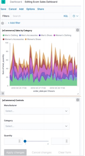
Inspecting Elements
We can inspect the Dashboard elements by choosing the visualizations panel menu and selecting Inspect. This will bring out the data behind the element which also can be downloaded.

Sharing Dashboard
We can share the dashboard by choosing the share menu and selecting the option to get a hyperlink as shown below −

Elasticsearch - Filtering by Field
The discover functionality available in Kibana home page allows us to explore the data sets from various angles. You can search and filter data for the selected index patterns. The data is usually available in form of distribution of values over a period of time.
To explore the ecommerce data sample, we click on the Discover icon as shown in the picture below. This will bring up the data along with the chart.
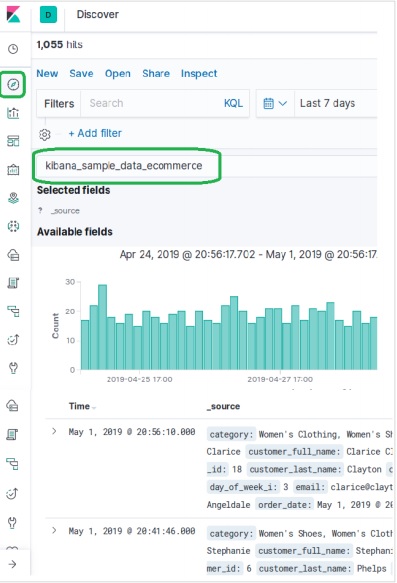
Filtering by Time
To filter out data by specific time interval we use the time filter option as shown below. By default, the filter is set at 15 minutes.
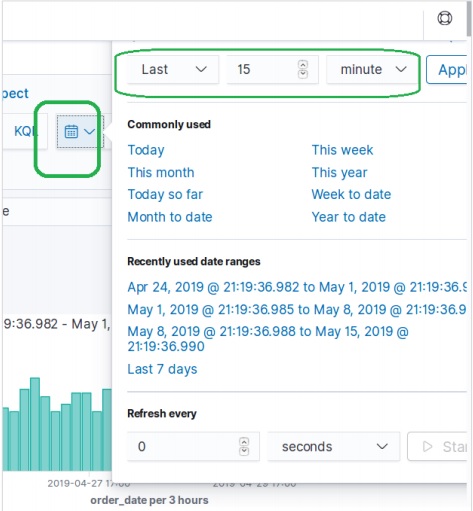
Filtering by Fields
The data set can also be filtered by fields using the Add Filter option as shown below. Here we add one or more fields and get the corresponding result after the filters are applied. In our example we choose the field day_of_week and then the operator for that field as is and value as Sunday.
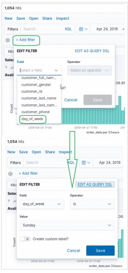
Next, we click Save with above filter conditions. The result set containing the filter conditions applied is shown below.
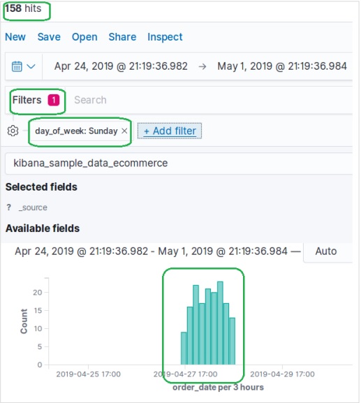
Elasticsearch - Data Tables
The data table is type of visualization that is used to display the raw data of a composed aggregation. There are various types of aggregations that are presented by using Data tables. In order to create a Data Table, we should go through the steps that are discussed here in detail.
Visualize
In Kibana Home screen we find the option name Visualize which allows us to create visualization and aggregations from the indices stored in Elasticsearch. The following image shows the option.
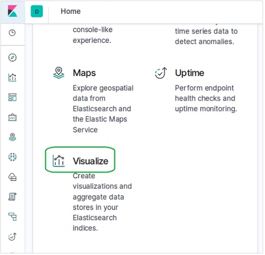
Select Data Table
Next, we select the Data Table option from among the various visualization options available. The option is shown in the following image &miuns;

Select Metrics
We then select the metrics needed for creating the data table visualization. This choice decides the type of aggregation we are going to use. We select the specific fields shown below from the ecommerce data set for this.
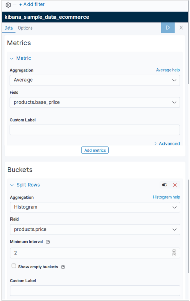
On running the above configuration for Data Table, we get the result as shown in the image here −
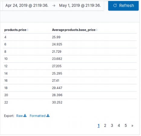
Elasticsearch - Region Maps
Region Maps show metrics on a geographic Map. It is useful in looking at the data anchored to different geographic regions with varying intensity. The darker shades usually indicate higher values and the lighter shades indicate lower values.
The steps to create this visualization are as explained in detail as follows −
Visualize
In this step we go to the visualize button available in the left bar of the Kibana Home screen and then choosing the option to add a new Visualization.
The following screen shows how we choose the region Map option.

Choose the Metrics
The next screen prompts us for choosing the metrics which will be used in creating the Region Map. Here we choose the Average price as the metric and country_iso_code as the field in the bucket which will be used in creating the visualization.
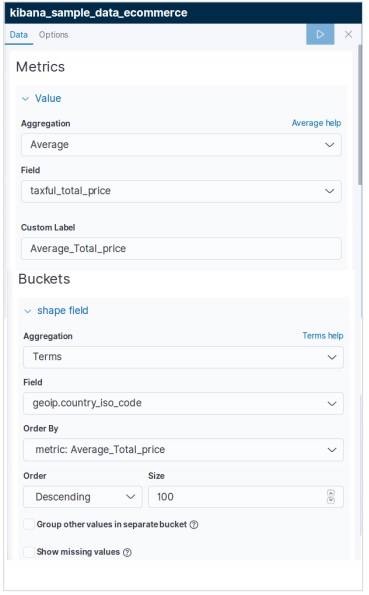
The final result below shows the Region Map once we apply the selection. Please note the shades of the colour and their values mentioned in the label.

Elasticsearch - Pie Charts
Pie charts are one of the simplest and famous visualization tools. It represents the data as slices of a circle each coloured differently. The labels along with the percentage data values can be presented along with the circle. The circle can also take the shape of a donut.
Visualize
In Kibana Home screen, we find the option name Visualize which allows us to create visualization and aggregations from the indices stored in Elasticsearch. We choose to add a new visualization and select pie chart as the option shown below.

Choose the Metrics
The next screen prompts us for choosing the metrics which will be used in creating the Pie Chart. Here we choose the count of base unit price as the metric and Bucket Aggregation as histogram. Also, the minimum interval is chosen as 20. So, the prices will be displayed as blocks of values with 20 as a range.
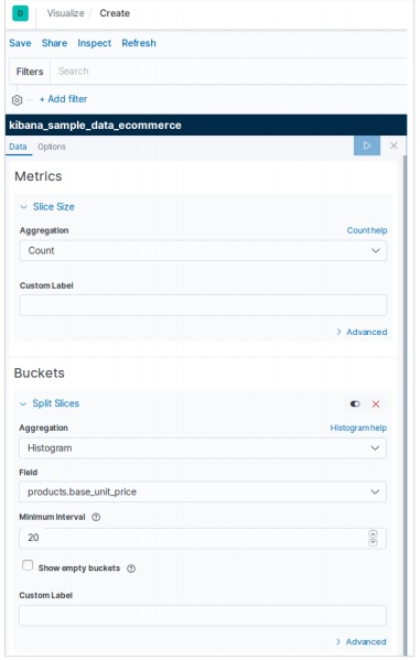
The result below shows the pie chart after we apply the selection. Please note the shades of the colour and their values mentioned in the label.

Pie Chart Options
On moving to the options tab under pie chart we can see various configuration options to change the look as well as the arrangement of data display in the pie chart. In the following example, the pie chart appears as donut and the labels appear at the top.
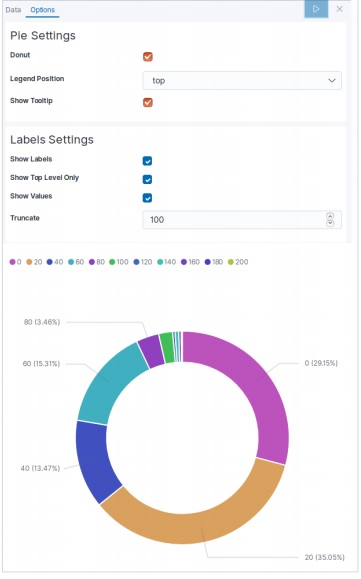
Elasticsearch - Area and Bar Charts
An area chart is an extension of line chart where the area between the line chart and the axes is highlighted with some colours. A bar chart represents data organized into a range of values and then plotted against the axes. It can consist of either horizontal bars or vertical bars.
In this chapter we will see all these three types of graphs that is created using Kibana. As discussed in earlier chapters we will continue to use the data in the ecommerce index.
Area Chart
In Kibana Home screen, we find the option name Visualize which allows us to create visualization and aggregations from the indices stored in Elasticsearch. We choose to add a new visualization and select Area Chart as the option shown in the image given below.

Choose the Metrics
The next screen prompts us for choosing the metrics which will be used in creating the Area Chart. Here we choose the sum as the type of aggregation metric. Then we choose total_quantity field as the field to be used as metric. On the X-axis, we chose the order_date field and split the series with the given metric in a size of 5.

On running the above configuration, we get the following area chart as the output −

Horizontal Bar Chart
Similarly, for the Horizontal bar chart we choose new visualization from Kibana Home screen and choose the option for Horizontal Bar. Then we choose the metrics as shown in the image below. Here we choose Sum as the aggregation for the filed named product quantity. Then we choose buckets with date histogram for the field order date.
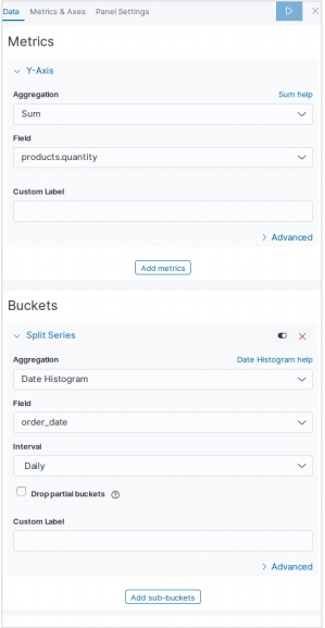
On running the above configuration, we can see a horizontal bar chart as shown below −

Vertical Bar Chart
For the vertical bar chart, we choose new visualization from Kibana Home screen and choose the option for Vertical Bar. Then we choose the metrics as shown in the image below.
Here we choose Sum as the aggregation for the field named product quantity. Then we choose buckets with date histogram for the field order date with a weekly interval.
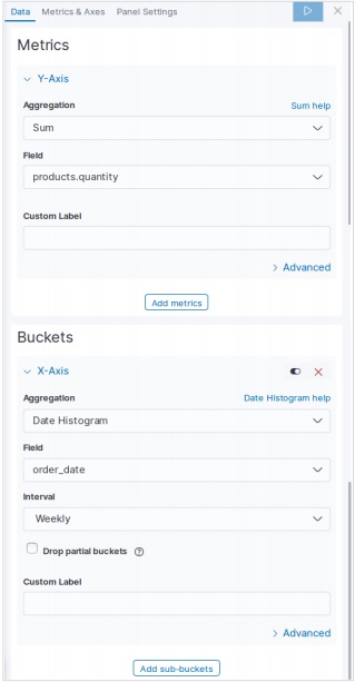
On running the above configuration, a chart will be generated as shown below −
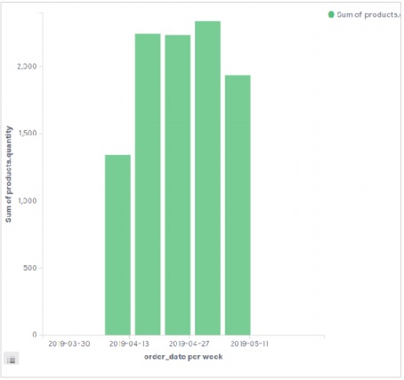
Elasticsearch - Time Series
Time series is a representation of sequence of data in a specific time sequence. For example, the data for each day starting from first day of the month to the last day. The interval between the data points remains constant. Any data set which has a time component in it can be represented as a time series.
In this chapter, we will use the sample e-commerce data set and plot the count of the number of orders for each day to create a time series.

Choose Metrics
First, we choose the index pattern, data field and interval which will be used for creating the time series. From the sample ecommerce data set we choose order_date as the field and 1d as the interval. We use the Panel Options tab to make these choices. Also we leave the other values in this tab as default to get a default colour and format for the time series.
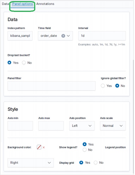
In the Data tab, we choose count as the aggregation option, group by option as everything and put a label for the time series chart.

Result
The final result of this configuration appears as follows. Please note that we are using a time period of Month to Date for this graph. Different time periods will give different results.
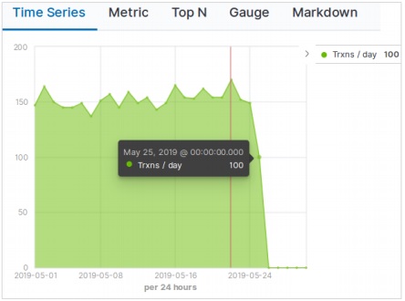
Elasticsearch - Tag Clouds
A tag cloud represents text which are mostly keywords and metadata in a visually appealing form. They are aligned in different angles and represented in different colours and font sizes. It helps in finding out the most prominent terms in the data. The prominence can be decided by one or more factors like frequency of the term, uniquness of the tag or based on some weightage attached to specific terms etc. Below we see the steps to create a Tag Cloud.
Visualize
In Kibana Home screen, we find the option name Visualize which allows us to create visualization and aggregations from the indices stored in Elasticsearch. We choose to add a new visualization and select Tag Cloud as the option shown below −

Choose the Metrics
The next screen prompts us for choosing the metrics which will be used in creating the Tag Cloud. Here we choose the count as the type of aggregation metric. Then we choose productname field as the keyword to be used as tags.
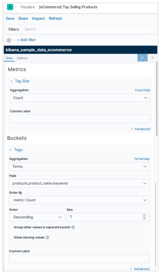
The result shown here shows the pie chart after we apply the selection. Please note the shades of the colour and their values mentioned in the label.

Tag Cloud Options
On moving to the options tab under Tag Cloud we can see various configuration options to change the look as well as the arrangement of data display in the Tag Cloud. In the below example the Tag Cloud appears with tags spread across both horizontal and vertical directions.

Elasticsearch - Heat Maps
Heat map is a type of visualization in which different shades of colour represent different areas in the graph. The values may be continuously varying and hence the colour r shades of a colour vary along with the values. They are very useful to represent both the continuously varying data as well as discrete data.
In this chapter we will use the data set named sample_data_flights to build a heatmap chart. In it we consider the variables named origin country and destination country of flights and take a count.
In Kibana Home screen, we find the option name Visualize which allows us to create visualization and aggregations from the indices stored in Elasticsearch. We choose to add a new visualization and select Heat Map as the option shown below &mimus;

Choose the Metrics
The next screen prompts us for choosing the metrics which will be used in creating the Heat Map Chart. Here we choose the count as the type of aggregation metric. Then for the buckets in Y-Axis, we choose Terms as the aggregation for the field OriginCountry. For the X-Axis, we choose the same aggregation but DestCountry as the field to be used. In both the cases, we choose the size of the bucket as 5.
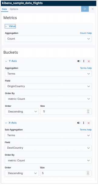
On running the above shown configuration, we get the heat map chart generated as follows.
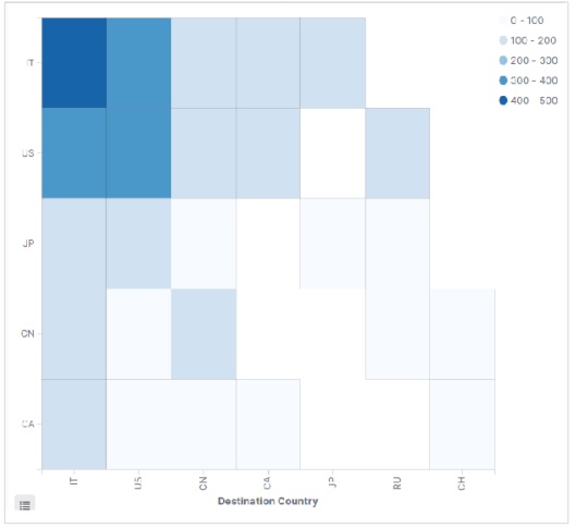
Note − You have to allow the date range as This Year so that the graph gathers data for a year to produce an effective heat map chart.
Elasticsearch - Canvas
Canvas application is a part of Kibana which allows us to create dynamic, multi-page and pixel perfect data displays. Its ability to create infographics and not just charts and metrices is what makes it unique and appealing. In this chapter we will see various features of canvas and how to use the canvas work pads.
Opening a Canvas
Go to the Kibana homepage and select the option as shown in the below diagram. It opens up the list of canvas work pads you have. We choose the ecommerce Revenue tracking for our study.
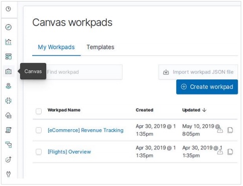
Cloning A Workpad
We clone the [eCommerce] Revenue Tracking workpad to be used in our study. To clone it, we highlight the row with the name of this workpad and then use the clone button as shown in the diagram below −
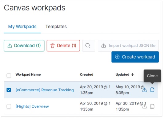
As a result of the above clone, we will get a new work pad named as [eCommerce] Revenue Tracking Copy which on opening will show the below infographics.
It describes the total sales and Revenue by category along with nice pictures and charts.

Modifying the Workpad
We can change the style and figures in the workpad by using the options available in the right hand side tab. Here we aim to change the background colour of the workpad by choosing a different colour as shown in the diagram below. The colour selection comes into effect immediately and we get the result as shown below −

Elasticsearch - Logs UI
Kibana can also help in visualizing log data from various sources. Logs are important sources of analysis for infrastructure health, performance needs and security breach analysis etc. Kibana can connect to various logs like web server logs, elasticsearch logs and cloudwatch logs etc.
Logstash Logs
In Kibana, we can connect to logstash logs for visualization. First we choose the Logs button from the Kibana home screen as shown below −
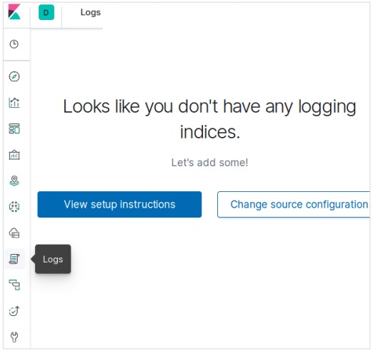
Then we choose the option Change Source Configuration which brings us the option to choose Logstash as a source. The below screen also shows other types of options we have as a log source.
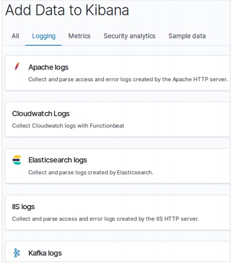
You can stream data for live log tailing or pause streaming to focus on historical log data. When you are streaming logs, the most recent log appears at the bottom on the console.
For further reference, you can refer to our Logstash tutorial.
