- Distributed Database Environments
- DDBMS - Design Strategies
- DDBMS - Distribution Transparency
- DDBMS - Database Control
- Query Optimization
- Relational Algebra Query
- Query Optimization Centralized
- Query Optimization in Distributed
- Concurrency Control
- Transaction Processing Systems
- DDBMS - Controlling Concurrency
- DDBMS - Deadlock Handling
- Failure and Recovery
- DDBMS - Replication Control
- DDBMS - Failure & Commit
- DDBMS - Database Recovery
- Distributed Commit Protocols
- Distributed DBMS Security
- Database Security & Cryptography
- Security in Distributed Databases
- Distributed DBMS Resources
- DDBMS - Quick Guide
- DDBMS - Useful Resources
- DDBMS - Discussion
Distributed DBMS - Quick Guide
Distributed DBMS - Concepts
For proper functioning of any organization, theres a need for a well-maintained database. In the recent past, databases used to be centralized in nature. However, with the increase in globalization, organizations tend to be diversified across the globe. They may choose to distribute data over local servers instead of a central database. Thus, arrived the concept of Distributed Databases.
This chapter gives an overview of databases and Database Management Systems (DBMS). A database is an ordered collection of related data. A DBMS is a software package to work upon a database. A detailed study of DBMS is available in our tutorial named Learn DBMS. In this chapter, we revise the main concepts so that the study of DDBMS can be done with ease. The three topics covered are database schemas, types of databases and operations on databases.
Database and Database Management System
A database is an ordered collection of related data that is built for a specific purpose. A database may be organized as a collection of multiple tables, where a table represents a real world element or entity. Each table has several different fields that represent the characteristic features of the entity.
For example, a company database may include tables for projects, employees, departments, products and financial records. The fields in the Employee table may be Name, Company_Id, Date_of_Joining, and so forth.
A database management system is a collection of programs that enables creation and maintenance of a database. DBMS is available as a software package that facilitates definition, construction, manipulation and sharing of data in a database. Definition of a database includes description of the structure of a database. Construction of a database involves actual storing of the data in any storage medium. Manipulation refers to the retrieving information from the database, updating the database and generating reports. Sharing of data facilitates data to be accessed by different users or programs.
Examples of DBMS Application Areas
- Automatic Teller Machines
- Train Reservation System
- Employee Management System
- Student Information System
Examples of DBMS Packages
- MySQL
- Oracle
- SQL Server
- dBASE
- FoxPro
- PostgreSQL, etc.
Database Schemas
A database schema is a description of the database which is specified during database design and subject to infrequent alterations. It defines the organization of the data, the relationships among them, and the constraints associated with them.
Databases are often represented through the three-schema architecture or ANSISPARC architecture. The goal of this architecture is to separate the user application from the physical database. The three levels are −
Internal Level having Internal Schema − It describes the physical structure, details of internal storage and access paths for the database.
Conceptual Level having Conceptual Schema − It describes the structure of the whole database while hiding the details of physical storage of data. This illustrates the entities, attributes with their data types and constraints, user operations and relationships.
External or View Level having External Schemas or Views − It describes the portion of a database relevant to a particular user or a group of users while hiding the rest of database.
Types of DBMS
There are four types of DBMS.
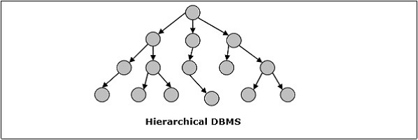
Hierarchical DBMS
In hierarchical DBMS, the relationships among data in the database are established so that one data element exists as a subordinate of another. The data elements have parent-child relationships and are modelled using the tree data structure. These are very fast and simple.
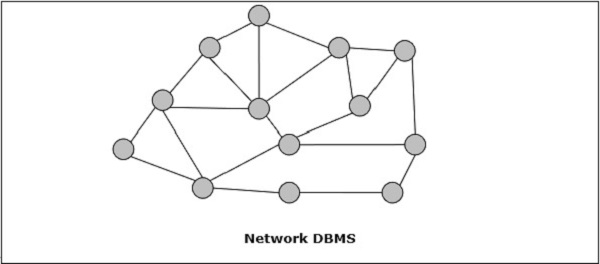
Network DBMS
Network DBMS in one where the relationships among data in the database are of type many-to-many in the form of a network. The structure is generally complicated due to the existence of numerous many-to-many relationships. Network DBMS is modelled using graph data structure.
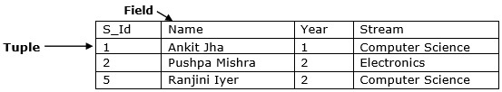
Relational DBMS
In relational databases, the database is represented in the form of relations. Each relation models an entity and is represented as a table of values. In the relation or table, a row is called a tuple and denotes a single record. A column is called a field or an attribute and denotes a characteristic property of the entity. RDBMS is the most popular database management system.
For example − A Student Relation −
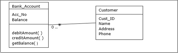
Object Oriented DBMS
Object-oriented DBMS is derived from the model of the object-oriented programming paradigm. They are helpful in representing both consistent data as stored in databases, as well as transient data, as found in executing programs. They use small, reusable elements called objects. Each object contains a data part and a set of operations which works upon the data. The object and its attributes are accessed through pointers instead of being stored in relational table models.
For example − A simplified Bank Account object-oriented database −
Distributed DBMS
A distributed database is a set of interconnected databases that is distributed over the computer network or internet. A Distributed Database Management System (DDBMS) manages the distributed database and provides mechanisms so as to make the databases transparent to the users. In these systems, data is intentionally distributed among multiple nodes so that all computing resources of the organization can be optimally used.
Operations on DBMS
The four basic operations on a database are Create, Retrieve, Update and Delete.
CREATE database structure and populate it with data − Creation of a database relation involves specifying the data structures, data types and the constraints of the data to be stored.
Example − SQL command to create a student table −
CREATE TABLE STUDENT (
   ROLL INTEGER PRIMARY KEY,
   NAME VARCHAR2(25),
   YEAR INTEGER,
   STREAM VARCHAR2(10)
);
Once the data format is defined, the actual data is stored in accordance with the format in some storage medium.
Example SQL command to insert a single tuple into the student table −
INSERT INTO STUDENT ( ROLL, NAME, YEAR, STREAM)
VALUES ( 1, 'ANKIT JHA', 1, 'COMPUTER SCIENCE');
RETRIEVE information from the database Retrieving information generally involves selecting a subset of a table or displaying data from the table after some computations have been done. It is done by querying upon the table.
Example − To retrieve the names of all students of the Computer Science stream, the following SQL query needs to be executed −
SELECT NAME FROM STUDENT
WHERE STREAM = 'COMPUTER SCIENCE';
UPDATE information stored and modify database structure Updating a table involves changing old values in the existing tables rows with new values.
Example − SQL command to change stream from Electronics to Electronics and Communications −
UPDATE STUDENT
SET STREAM = 'ELECTRONICS AND COMMUNICATIONS'
WHERE STREAM = 'ELECTRONICS';
Modifying database means to change the structure of the table. However, modification of the table is subject to a number of restrictions.
Example − To add a new field or column, say address to the Student table, we use the following SQL command −
ALTER TABLE STUDENT
ADD ( ADDRESS VARCHAR2(50) );
DELETE information stored or delete a table as a whole Deletion of specific information involves removal of selected rows from the table that satisfies certain conditions.
Example − To delete all students who are in 4th year currently when they are passing out, we use the SQL command −
DELETE FROM STUDENT
WHERE YEAR = 4;
Alternatively, the whole table may be removed from the database.
Example − To remove the student table completely, the SQL command used is −
DROP TABLE STUDENT;
Distributed DBMS - Distributed Databases
This chapter introduces the concept of DDBMS. In a distributed database, there are a number of databases that may be geographically distributed all over the world. A distributed DBMS manages the distributed database in a manner so that it appears as one single database to users. In the later part of the chapter, we go on to study the factors that lead to distributed databases, its advantages and disadvantages.
A distributed database is a collection of multiple interconnected databases, which are spread physically across various locations that communicate via a computer network.
Features
Databases in the collection are logically interrelated with each other. Often they represent a single logical database.
Data is physically stored across multiple sites. Data in each site can be managed by a DBMS independent of the other sites.
The processors in the sites are connected via a network. They do not have any multiprocessor configuration.
A distributed database is not a loosely connected file system.
A distributed database incorporates transaction processing, but it is not synonymous with a transaction processing system.
Distributed Database Management System
A distributed database management system (DDBMS) is a centralized software system that manages a distributed database in a manner as if it were all stored in a single location.
Features
It is used to create, retrieve, update and delete distributed databases.
It synchronizes the database periodically and provides access mechanisms by the virtue of which the distribution becomes transparent to the users.
It ensures that the data modified at any site is universally updated.
It is used in application areas where large volumes of data are processed and accessed by numerous users simultaneously.
It is designed for heterogeneous database platforms.
It maintains confidentiality and data integrity of the databases.
Factors Encouraging DDBMS
The following factors encourage moving over to DDBMS −
Distributed Nature of Organizational Units − Most organizations in the current times are subdivided into multiple units that are physically distributed over the globe. Each unit requires its own set of local data. Thus, the overall database of the organization becomes distributed.
Need for Sharing of Data − The multiple organizational units often need to communicate with each other and share their data and resources. This demands common databases or replicated databases that should be used in a synchronized manner.
Support for Both OLTP and OLAP − Online Transaction Processing (OLTP) and Online Analytical Processing (OLAP) work upon diversified systems which may have common data. Distributed database systems aid both these processing by providing synchronized data.
Database Recovery − One of the common techniques used in DDBMS is replication of data across different sites. Replication of data automatically helps in data recovery if database in any site is damaged. Users can access data from other sites while the damaged site is being reconstructed. Thus, database failure may become almost inconspicuous to users.
Support for Multiple Application Software − Most organizations use a variety of application software each with its specific database support. DDBMS provides a uniform functionality for using the same data among different platforms.
Advantages of Distributed Databases
Following are the advantages of distributed databases over centralized databases.
Modular Development − If the system needs to be expanded to new locations or new units, in centralized database systems, the action requires substantial efforts and disruption in the existing functioning. However, in distributed databases, the work simply requires adding new computers and local data to the new site and finally connecting them to the distributed system, with no interruption in current functions.
More Reliable − In case of database failures, the total system of centralized databases comes to a halt. However, in distributed systems, when a component fails, the functioning of the system continues may be at a reduced performance. Hence DDBMS is more reliable.
Better Response − If data is distributed in an efficient manner, then user requests can be met from local data itself, thus providing faster response. On the other hand, in centralized systems, all queries have to pass through the central computer for processing, which increases the response time.
Lower Communication Cost − In distributed database systems, if data is located locally where it is mostly used, then the communication costs for data manipulation can be minimized. This is not feasible in centralized systems.
Adversities of Distributed Databases
Following are some of the adversities associated with distributed databases.
Need for complex and expensive software − DDBMS demands complex and often expensive software to provide data transparency and co-ordination across the several sites.
Processing overhead − Even simple operations may require a large number of communications and additional calculations to provide uniformity in data across the sites.
Data integrity − The need for updating data in multiple sites pose problems of data integrity.
Overheads for improper data distribution − Responsiveness of queries is largely dependent upon proper data distribution. Improper data distribution often leads to very slow response to user requests.
Distributed DBMS - Database Environments
In this part of the tutorial, we will study the different aspects that aid in designing distributed database environments. This chapter starts with the types of distributed databases. Distributed databases can be classified into homogeneous and heterogeneous databases having further divisions. The next section of this chapter discusses the distributed architectures namely client server, peer to peer and multi DBMS. Finally, the different design alternatives like replication and fragmentation are introduced.
Types of Distributed Databases
Distributed databases can be broadly classified into homogeneous and heterogeneous distributed database environments, each with further sub-divisions, as shown in the following illustration.
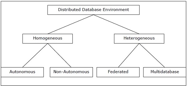
Homogeneous Distributed Databases
In a homogeneous distributed database, all the sites use identical DBMS and operating systems. Its properties are −
The sites use very similar software.
The sites use identical DBMS or DBMS from the same vendor.
Each site is aware of all other sites and cooperates with other sites to process user requests.
The database is accessed through a single interface as if it is a single database.
Types of Homogeneous Distributed Database
There are two types of homogeneous distributed database −
Autonomous − Each database is independent that functions on its own. They are integrated by a controlling application and use message passing to share data updates.
Non-autonomous − Data is distributed across the homogeneous nodes and a central or master DBMS co-ordinates data updates across the sites.
Heterogeneous Distributed Databases
In a heterogeneous distributed database, different sites have different operating systems, DBMS products and data models. Its properties are −
Different sites use dissimilar schemas and software.
The system may be composed of a variety of DBMSs like relational, network, hierarchical or object oriented.
Query processing is complex due to dissimilar schemas.
Transaction processing is complex due to dissimilar software.
A site may not be aware of other sites and so there is limited co-operation in processing user requests.
Types of Heterogeneous Distributed Databases
Federated − The heterogeneous database systems are independent in nature and integrated together so that they function as a single database system.
Un-federated − The database systems employ a central coordinating module through which the databases are accessed.
Distributed DBMS Architectures
DDBMS architectures are generally developed depending on three parameters −
Distribution − It states the physical distribution of data across the different sites.
Autonomy − It indicates the distribution of control of the database system and the degree to which each constituent DBMS can operate independently.
Heterogeneity − It refers to the uniformity or dissimilarity of the data models, system components and databases.
Architectural Models
Some of the common architectural models are −
- Client - Server Architecture for DDBMS
- Peer - to - Peer Architecture for DDBMS
- Multi - DBMS Architecture
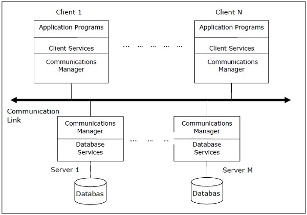
Client - Server Architecture for DDBMS
This is a two-level architecture where the functionality is divided into servers and clients. The server functions primarily encompass data management, query processing, optimization and transaction management. Client functions include mainly user interface. However, they have some functions like consistency checking and transaction management.
The two different client - server architecture are −
- Single Server Multiple Client
- Multiple Server Multiple Client (shown in the following diagram)
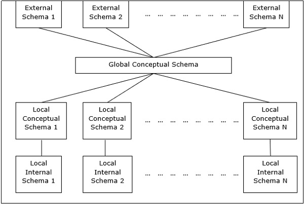
Peer- to-Peer Architecture for DDBMS
In these systems, each peer acts both as a client and a server for imparting database services. The peers share their resource with other peers and co-ordinate their activities.
This architecture generally has four levels of schemas −
Global Conceptual Schema − Depicts the global logical view of data.
Local Conceptual Schema − Depicts logical data organization at each site.
Local Internal Schema − Depicts physical data organization at each site.
External Schema − Depicts user view of data.
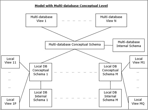
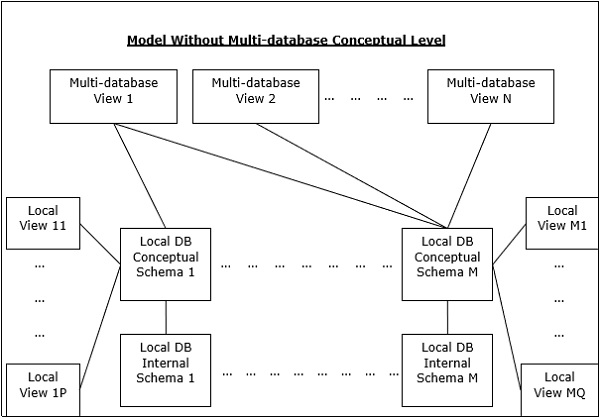
Multi - DBMS Architectures
This is an integrated database system formed by a collection of two or more autonomous database systems.
Multi-DBMS can be expressed through six levels of schemas −
Multi-database View Level − Depicts multiple user views comprising of subsets of the integrated distributed database.
Multi-database Conceptual Level − Depicts integrated multi-database that comprises of global logical multi-database structure definitions.
Multi-database Internal Level − Depicts the data distribution across different sites and multi-database to local data mapping.
Local database View Level − Depicts public view of local data.
Local database Conceptual Level − Depicts local data organization at each site.
Local database Internal Level − Depicts physical data organization at each site.
There are two design alternatives for multi-DBMS −
- Model with multi-database conceptual level.
- Model without multi-database conceptual level.
Design Alternatives
The distribution design alternatives for the tables in a DDBMS are as follows −
- Non-replicated and non-fragmented
- Fully replicated
- Partially replicated
- Fragmented
- Mixed
Non-replicated & Non-fragmented
In this design alternative, different tables are placed at different sites. Data is placed so that it is at a close proximity to the site where it is used most. It is most suitable for database systems where the percentage of queries needed to join information in tables placed at different sites is low. If an appropriate distribution strategy is adopted, then this design alternative helps to reduce the communication cost during data processing.
Fully Replicated
In this design alternative, at each site, one copy of all the database tables is stored. Since, each site has its own copy of the entire database, queries are very fast requiring negligible communication cost. On the contrary, the massive redundancy in data requires huge cost during update operations. Hence, this is suitable for systems where a large number of queries is required to be handled whereas the number of database updates is low.
Partially Replicated
Copies of tables or portions of tables are stored at different sites. The distribution of the tables is done in accordance to the frequency of access. This takes into consideration the fact that the frequency of accessing the tables vary considerably from site to site. The number of copies of the tables (or portions) depends on how frequently the access queries execute and the site which generate the access queries.
Fragmented
In this design, a table is divided into two or more pieces referred to as fragments or partitions, and each fragment can be stored at different sites. This considers the fact that it seldom happens that all data stored in a table is required at a given site. Moreover, fragmentation increases parallelism and provides better disaster recovery. Here, there is only one copy of each fragment in the system, i.e. no redundant data.
The three fragmentation techniques are −
- Vertical fragmentation
- Horizontal fragmentation
- Hybrid fragmentation
Mixed Distribution
This is a combination of fragmentation and partial replications. Here, the tables are initially fragmented in any form (horizontal or vertical), and then these fragments are partially replicated across the different sites according to the frequency of accessing the fragments.
Distributed DBMS - Design Strategies
In the last chapter, we had introduced different design alternatives. In this chapter, we will study the strategies that aid in adopting the designs. The strategies can be broadly divided into replication and fragmentation. However, in most cases, a combination of the two is used.
Data Replication
Data replication is the process of storing separate copies of the database at two or more sites. It is a popular fault tolerance technique of distributed databases.
Advantages of Data Replication
Reliability − In case of failure of any site, the database system continues to work since a copy is available at another site(s).
Reduction in Network Load − Since local copies of data are available, query processing can be done with reduced network usage, particularly during prime hours. Data updating can be done at non-prime hours.
Quicker Response − Availability of local copies of data ensures quick query processing and consequently quick response time.
Simpler Transactions − Transactions require less number of joins of tables located at different sites and minimal coordination across the network. Thus, they become simpler in nature.
Disadvantages of Data Replication
Increased Storage Requirements − Maintaining multiple copies of data is associated with increased storage costs. The storage space required is in multiples of the storage required for a centralized system.
Increased Cost and Complexity of Data Updating − Each time a data item is updated, the update needs to be reflected in all the copies of the data at the different sites. This requires complex synchronization techniques and protocols.
Undesirable Application Database coupling − If complex update mechanisms are not used, removing data inconsistency requires complex co-ordination at application level. This results in undesirable application database coupling.
Some commonly used replication techniques are −
- Snapshot replication
- Near-real-time replication
- Pull replication
Fragmentation
Fragmentation is the task of dividing a table into a set of smaller tables. The subsets of the table are called fragments. Fragmentation can be of three types: horizontal, vertical, and hybrid (combination of horizontal and vertical). Horizontal fragmentation can further be classified into two techniques: primary horizontal fragmentation and derived horizontal fragmentation.
Fragmentation should be done in a way so that the original table can be reconstructed from the fragments. This is needed so that the original table can be reconstructed from the fragments whenever required. This requirement is called reconstructiveness.
Advantages of Fragmentation
Since data is stored close to the site of usage, efficiency of the database system is increased.
Local query optimization techniques are sufficient for most queries since data is locally available.
Since irrelevant data is not available at the sites, security and privacy of the database system can be maintained.
Disadvantages of Fragmentation
When data from different fragments are required, the access speeds may be very low.
In case of recursive fragmentations, the job of reconstruction will need expensive techniques.
Lack of back-up copies of data in different sites may render the database ineffective in case of failure of a site.
Vertical Fragmentation
In vertical fragmentation, the fields or columns of a table are grouped into fragments. In order to maintain reconstructiveness, each fragment should contain the primary key field(s) of the table. Vertical fragmentation can be used to enforce privacy of data.
For example, let us consider that a University database keeps records of all registered students in a Student table having the following schema.
STUDENT
| Regd_No | Name | Course | Address | Semester | Fees | Marks |
Now, the fees details are maintained in the accounts section. In this case, the designer will fragment the database as follows −
CREATE TABLE STD_FEES AS
   SELECT Regd_No, Fees
   FROM STUDENT;
Horizontal Fragmentation
Horizontal fragmentation groups the tuples of a table in accordance to values of one or more fields. Horizontal fragmentation should also confirm to the rule of reconstructiveness. Each horizontal fragment must have all columns of the original base table.
For example, in the student schema, if the details of all students of Computer Science Course needs to be maintained at the School of Computer Science, then the designer will horizontally fragment the database as follows −
CREATE COMP_STD AS
   SELECT * FROM STUDENT
   WHERE COURSE = "Computer Science";
Hybrid Fragmentation
In hybrid fragmentation, a combination of horizontal and vertical fragmentation techniques are used. This is the most flexible fragmentation technique since it generates fragments with minimal extraneous information. However, reconstruction of the original table is often an expensive task.
Hybrid fragmentation can be done in two alternative ways −
At first, generate a set of horizontal fragments; then generate vertical fragments from one or more of the horizontal fragments.
At first, generate a set of vertical fragments; then generate horizontal fragments from one or more of the vertical fragments.
DDBMS - Distribution Transparency
Distribution transparency is the property of distributed databases by the virtue of which the internal details of the distribution are hidden from the users. The DDBMS designer may choose to fragment tables, replicate the fragments and store them at different sites. However, since users are oblivious of these details, they find the distributed database easy to use like any centralized database.
The three dimensions of distribution transparency are −
- Location transparency
- Fragmentation transparency
- Replication transparency
Location Transparency
Location transparency ensures that the user can query on any table(s) or fragment(s) of a table as if they were stored locally in the users site. The fact that the table or its fragments are stored at remote site in the distributed database system, should be completely oblivious to the end user. The address of the remote site(s) and the access mechanisms are completely hidden.
In order to incorporate location transparency, DDBMS should have access to updated and accurate data dictionary and DDBMS directory which contains the details of locations of data.
Fragmentation Transparency
Fragmentation transparency enables users to query upon any table as if it were unfragmented. Thus, it hides the fact that the table the user is querying on is actually a fragment or union of some fragments. It also conceals the fact that the fragments are located at diverse sites.
This is somewhat similar to users of SQL views, where the user may not know that they are using a view of a table instead of the table itself.
Replication Transparency
Replication transparency ensures that replication of databases are hidden from the users. It enables users to query upon a table as if only a single copy of the table exists.
Replication transparency is associated with concurrency transparency and failure transparency. Whenever a user updates a data item, the update is reflected in all the copies of the table. However, this operation should not be known to the user. This is concurrency transparency. Also, in case of failure of a site, the user can still proceed with his queries using replicated copies without any knowledge of failure. This is failure transparency.
Combination of Transparencies
In any distributed database system, the designer should ensure that all the stated transparencies are maintained to a considerable extent. The designer may choose to fragment tables, replicate them and store them at different sites; all oblivious to the end user. However, complete distribution transparency is a tough task and requires considerable design efforts.
Distributed DBMS - Database Control
Database control refers to the task of enforcing regulations so as to provide correct data to authentic users and applications of a database. In order that correct data is available to users, all data should conform to the integrity constraints defined in the database. Besides, data should be screened away from unauthorized users so as to maintain security and privacy of the database. Database control is one of the primary tasks of the database administrator (DBA).
The three dimensions of database control are −
- Authentication
- Access rights
- Integrity constraints
Authentication
In a distributed database system, authentication is the process through which only legitimate users can gain access to the data resources.
Authentication can be enforced in two levels −
Controlling Access to Client Computer − At this level, user access is restricted while login to the client computer that provides user-interface to the database server. The most common method is a username/password combination. However, more sophisticated methods like biometric authentication may be used for high security data.
Controlling Access to the Database Software − At this level, the database software/administrator assigns some credentials to the user. The user gains access to the database using these credentials. One of the methods is to create a login account within the database server.
Access Rights
A users access rights refers to the privileges that the user is given regarding DBMS operations such as the rights to create a table, drop a table, add/delete/update tuples in a table or query upon the table.
In distributed environments, since there are large number of tables and yet larger number of users, it is not feasible to assign individual access rights to users. So, DDBMS defines certain roles. A role is a construct with certain privileges within a database system. Once the different roles are defined, the individual users are assigned one of these roles. Often a hierarchy of roles are defined according to the organizations hierarchy of authority and responsibility.
For example, the following SQL statements create a role "Accountant" and then assigns this role to user "ABC".
CREATE ROLE ACCOUNTANT;
GRANT SELECT, INSERT, UPDATE ON EMP_SAL TO ACCOUNTANT;
GRANT INSERT, UPDATE, DELETE ON TENDER TO ACCOUNTANT;
GRANT INSERT, SELECT ON EXPENSE TO ACCOUNTANT;
COMMIT;
GRANT ACCOUNTANT TO ABC;
COMMIT;
Semantic Integrity Control
Semantic integrity control defines and enforces the integrity constraints of the database system.
The integrity constraints are as follows −
- Data type integrity constraint
- Entity integrity constraint
- Referential integrity constraint
Data Type Integrity Constraint
A data type constraint restricts the range of values and the type of operations that can be applied to the field with the specified data type.
For example, let us consider that a table "HOSTEL" has three fields - the hostel number, hostel name and capacity. The hostel number should start with capital letter "H" and cannot be NULL, and the capacity should not be more than 150. The following SQL command can be used for data definition −
CREATE TABLE HOSTEL (
   H_NO VARCHAR2(5) NOT NULL,
   H_NAME VARCHAR2(15),
   CAPACITY INTEGER,
   CHECK ( H_NO LIKE 'H%'),
   CHECK ( CAPACITY <= 150)
);
Entity Integrity Control
Entity integrity control enforces the rules so that each tuple can be uniquely identified from other tuples. For this a primary key is defined. A primary key is a set of minimal fields that can uniquely identify a tuple. Entity integrity constraint states that no two tuples in a table can have identical values for primary keys and that no field which is a part of the primary key can have NULL value.
For example, in the above hostel table, the hostel number can be assigned as the primary key through the following SQL statement (ignoring the checks) −
CREATE TABLE HOSTEL (
   H_NO VARCHAR2(5) PRIMARY KEY,
   H_NAME VARCHAR2(15),
   CAPACITY INTEGER
);
Referential Integrity Constraint
Referential integrity constraint lays down the rules of foreign keys. A foreign key is a field in a data table that is the primary key of a related table. The referential integrity constraint lays down the rule that the value of the foreign key field should either be among the values of the primary key of the referenced table or be entirely NULL.
For example, let us consider a student table where a student may opt to live in a hostel. To include this, the primary key of hostel table should be included as a foreign key in the student table. The following SQL statement incorporates this −
CREATE TABLE STUDENT (
   S_ROLL INTEGER PRIMARY KEY,
   S_NAME VARCHAR2(25) NOT NULL,
   S_COURSE VARCHAR2(10),
   S_HOSTEL VARCHAR2(5) REFERENCES HOSTEL
);
Relational Algebra for Query Optimization
When a query is placed, it is at first scanned, parsed and validated. An internal representation of the query is then created such as a query tree or a query graph. Then alternative execution strategies are devised for retrieving results from the database tables. The process of choosing the most appropriate execution strategy for query processing is called query optimization.
Query Optimization Issues in DDBMS
In DDBMS, query optimization is a crucial task. The complexity is high since number of alternative strategies may increase exponentially due to the following factors −
- The presence of a number of fragments.
- Distribution of the fragments or tables across various sites.
- The speed of communication links.
- Disparity in local processing capabilities.
Hence, in a distributed system, the target is often to find a good execution strategy for query processing rather than the best one. The time to execute a query is the sum of the following −
- Time to communicate queries to databases.
- Time to execute local query fragments.
- Time to assemble data from different sites.
- Time to display results to the application.
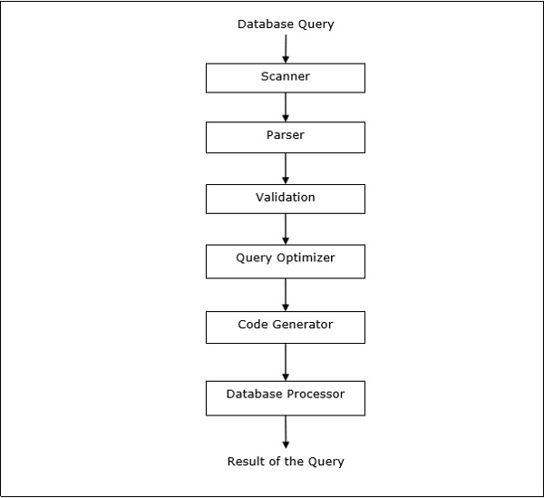
Query Processing
Query processing is a set of all activities starting from query placement to displaying the results of the query. The steps are as shown in the following diagram −
Relational Algebra
Relational algebra defines the basic set of operations of relational database model. A sequence of relational algebra operations forms a relational algebra expression. The result of this expression represents the result of a database query.
The basic operations are −
- Projection
- Selection
- Union
- Intersection
- Minus
- Join
Projection
Projection operation displays a subset of fields of a table. This gives a vertical partition of the table.
Syntax in Relational Algebra
$$\pi_{}{()}$$
For example, let us consider the following Student database −
| Roll_No | Name | Course | Semester | Gender |
| 2 | Amit Prasad | BCA | 1 | Male |
| 4 | Varsha Tiwari | BCA | 1 | Female |
| 5 | Asif Ali | MCA | 2 | Male |
| 6 | Joe Wallace | MCA | 1 | Male |
| 8 | Shivani Iyengar | BCA | 1 | Female |
If we want to display the names and courses of all students, we will use the following relational algebra expression −
$$\pi_{Name,Course}{(STUDENT)}$$
Selection
Selection operation displays a subset of tuples of a table that satisfies certain conditions. This gives a horizontal partition of the table.
Syntax in Relational Algebra
$$\sigma_{}{()}$$
For example, in the Student table, if we want to display the details of all students who have opted for MCA course, we will use the following relational algebra expression −
$$\sigma_{Course} = {\small "BCA"}^{(STUDENT)}$$
Combination of Projection and Selection Operations
For most queries, we need a combination of projection and selection operations. There are two ways to write these expressions −
- Using sequence of projection and selection operations.
- Using rename operation to generate intermediate results.
For example, to display names of all female students of the BCA course −
- Relational algebra expression using sequence of projection and selection operations
$$\pi_{Name}(\sigma_{Gender = \small "Female" AND \: Course = \small "BCA"}{(STUDENT)})$$
- Relational algebra expression using rename operation to generate intermediate results
$$FemaleBCAStudent \leftarrow \sigma_{Gender = \small "Female" AND \: Course = \small "BCA"} {(STUDENT)}$$
$$Result \leftarrow \pi_{Name}{(FemaleBCAStudent)}$$
Union
If P is a result of an operation and Q is a result of another operation, the union of P and Q ($p \cup Q$) is the set of all tuples that is either in P or in Q or in both without duplicates.
For example, to display all students who are either in Semester 1 or are in BCA course −
$$Sem1Student \leftarrow \sigma_{Semester = 1}{(STUDENT)}$$
$$BCAStudent \leftarrow \sigma_{Course = \small "BCA"}{(STUDENT)}$$
$$Result \leftarrow Sem1Student \cup BCAStudent$$
Intersection
If P is a result of an operation and Q is a result of another operation, the intersection of P and Q ( $p \cap Q$ ) is the set of all tuples that are in P and Q both.
For example, given the following two schemas −
EMPLOYEE
| EmpID | Name | City | Department | Salary |
PROJECT
| PId | City | Department | Status |
To display the names of all cities where a project is located and also an employee resides −
$$CityEmp \leftarrow \pi_{City}{(EMPLOYEE)}$$
$$CityProject \leftarrow \pi_{City}{(PROJECT)}$$
$$Result \leftarrow CityEmp \cap CityProject$$
Minus
If P is a result of an operation and Q is a result of another operation, P - Q is the set of all tuples that are in P and not in Q.
For example, to list all the departments which do not have an ongoing project (projects with status = ongoing) −
$$AllDept \leftarrow \pi_{Department}{(EMPLOYEE)}$$
$$ProjectDept \leftarrow \pi_{Department} (\sigma_{Status = \small "ongoing"}{(PROJECT)})$$
$$Result \leftarrow AllDept - ProjectDept$$
Join
Join operation combines related tuples of two different tables (results of queries) into a single table.
For example, consider two schemas, Customer and Branch in a Bank database as follows −
CUSTOMER
| CustID | AccNo | TypeOfAc | BranchID | DateOfOpening |
BRANCH
| BranchID | BranchName | IFSCcode | Address |
To list the employee details along with branch details −
$$Result \leftarrow CUSTOMER \bowtie_{Customer.BranchID=Branch.BranchID}{BRANCH}$$
Translating SQL Queries into Relational Algebra
SQL queries are translated into equivalent relational algebra expressions before optimization. A query is at first decomposed into smaller query blocks. These blocks are translated to equivalent relational algebra expressions. Optimization includes optimization of each block and then optimization of the query as a whole.
Examples
Let us consider the following schemas −
EMPLOYEE
| EmpID | Name | City | Department | Salary |
PROJECT
| PId | City | Department | Status |
WORKS
| EmpID | PID | Hours |
Example 1
To display the details of all employees who earn a salary LESS than the average salary, we write the SQL query −
SELECT * FROM EMPLOYEE
WHERE SALARY < ( SELECT AVERAGE(SALARY) FROM EMPLOYEE ) ;
This query contains one nested sub-query. So, this can be broken down into two blocks.
The inner block is −
SELECT AVERAGE(SALARY)FROM EMPLOYEE ;
If the result of this query is AvgSal, then outer block is −
SELECT * FROM EMPLOYEE WHERE SALARY < AvgSal;
Relational algebra expression for inner block −
$$AvgSal \leftarrow \Im_{AVERAGE(Salary)}{EMPLOYEE}$$
Relational algebra expression for outer block −
$$\sigma_{Salary }{EMPLOYEE}$$
Example 2
To display the project ID and status of all projects of employee 'Arun Kumar', we write the SQL query −
SELECT PID, STATUS FROM PROJECT
WHERE PID = ( SELECT FROM WORKS  WHERE EMPID = ( SELECT EMPID FROM EMPLOYEE
            WHERE NAME = 'ARUN KUMAR'));
This query contains two nested sub-queries. Thus, can be broken down into three blocks, as follows −
SELECT EMPID FROM EMPLOYEE WHERE NAME = 'ARUN KUMAR';
SELECT PID FROM WORKS WHERE EMPID = ArunEmpID;
SELECT PID, STATUS FROM PROJECT WHERE PID = ArunPID;
(Here ArunEmpID and ArunPID are the results of inner queries)
Relational algebra expressions for the three blocks are −
$$ArunEmpID \leftarrow \pi_{EmpID}(\sigma_{Name = \small "Arun Kumar"} {(EMPLOYEE)})$$
$$ArunPID \leftarrow \pi_{PID}(\sigma_{EmpID = \small "ArunEmpID"} {(WORKS)})$$
$$Result \leftarrow \pi_{PID, Status}(\sigma_{PID = \small "ArunPID"} {(PROJECT)})$$
Computation of Relational Algebra Operators
The computation of relational algebra operators can be done in many different ways, and each alternative is called an access path.
The computation alternative depends upon three main factors −
- Operator type
- Available memory
- Disk structures
The time to perform execution of a relational algebra operation is the sum of −
- Time to process the tuples.
- Time to fetch the tuples of the table from disk to memory.
Since the time to process a tuple is very much smaller than the time to fetch the tuple from the storage, particularly in a distributed system, disk access is very often considered as the metric for calculating cost of relational expression.
Computation of Selection
Computation of selection operation depends upon the complexity of the selection condition and the availability of indexes on the attributes of the table.
Following are the computation alternatives depending upon the indexes −
No Index − If the table is unsorted and has no indexes, then the selection process involves scanning all the disk blocks of the table. Each block is brought into the memory and each tuple in the block is examined to see whether it satisfies the selection condition. If the condition is satisfied, it is displayed as output. This is the costliest approach since each tuple is brought into memory and each tuple is processed.
B+ Tree Index − Most database systems are built upon the B+ Tree index. If the selection condition is based upon the field, which is the key of this B+ Tree index, then this index is used for retrieving results. However, processing selection statements with complex conditions may involve a larger number of disk block accesses and in some cases complete scanning of the table.
Hash Index − If hash indexes are used and its key field is used in the selection condition, then retrieving tuples using the hash index becomes a simple process. A hash index uses a hash function to find the address of a bucket where the key value corresponding to the hash value is stored. In order to find a key value in the index, the hash function is executed and the bucket address is found. The key values in the bucket are searched. If a match is found, the actual tuple is fetched from the disk block into the memory.
Computation of Joins
When we want to join two tables, say P and Q, each tuple in P has to be compared with each tuple in Q to test if the join condition is satisfied. If the condition is satisfied, the corresponding tuples are concatenated, eliminating duplicate fields and appended to the result relation. Consequently, this is the most expensive operation.
The common approaches for computing joins are −
Nested-loop Approach
This is the conventional join approach. It can be illustrated through the following pseudocode (Tables P and Q, with tuples tuple_p and tuple_q and joining attribute a) −
For each tuple_p in P
For each tuple_q in Q
If tuple_p.a = tuple_q.a Then
   Concatenate tuple_p and tuple_q and append to Result
End If
Next tuple_q
Next tuple-p
Sort-merge Approach
In this approach, the two tables are individually sorted based upon the joining attribute and then the sorted tables are merged. External sorting techniques are adopted since the number of records is very high and cannot be accommodated in the memory. Once the individual tables are sorted, one page each of the sorted tables are brought to the memory, merged based upon the joining attribute and the joined tuples are written out.
Hash-join Approach
This approach comprises of two phases: partitioning phase and probing phase. In partitioning phase, the tables P and Q are broken into two sets of disjoint partitions. A common hash function is decided upon. This hash function is used to assign tuples to partitions. In the probing phase, tuples in a partition of P are compared with the tuples of corresponding partition of Q. If they match, then they are written out.
Query Optimization in Centralized Systems
Once the alternative access paths for computation of a relational algebra expression are derived, the optimal access path is determined. In this chapter, we will look into query optimization in centralized system while in the next chapter we will study query optimization in a distributed system.
In a centralized system, query processing is done with the following aim −
Minimization of response time of query (time taken to produce the results to users query).
Maximize system throughput (the number of requests that are processed in a given amount of time).
Reduce the amount of memory and storage required for processing.
Increase parallelism.
Query Parsing and Translation
Initially, the SQL query is scanned. Then it is parsed to look for syntactical errors and correctness of data types. If the query passes this step, the query is decomposed into smaller query blocks. Each block is then translated to equivalent relational algebra expression.
Steps for Query Optimization
Query optimization involves three steps, namely query tree generation, plan generation, and query plan code generation.
Step 1 − Query Tree Generation
A query tree is a tree data structure representing a relational algebra expression. The tables of the query are represented as leaf nodes. The relational algebra operations are represented as the internal nodes. The root represents the query as a whole.
During execution, an internal node is executed whenever its operand tables are available. The node is then replaced by the result table. This process continues for all internal nodes until the root node is executed and replaced by the result table.
For example, let us consider the following schemas −
EMPLOYEE
| EmpID | EName | Salary | DeptNo | DateOfJoining |
DEPARTMENT
| DNo | DName | Location |
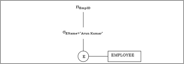
Example 1
Let us consider the query as the following.
$$\pi_{EmpID} (\sigma_{EName = \small "ArunKumar"} {(EMPLOYEE)})$$
The corresponding query tree will be −
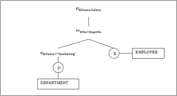
Example 2
Let us consider another query involving a join.
$\pi_{EName, Salary} (\sigma_{DName = \small "Marketing"} {(DEPARTMENT)}) \bowtie_{DNo=DeptNo}{(EMPLOYEE)}$
Following is the query tree for the above query.
Step 2 − Query Plan Generation
After the query tree is generated, a query plan is made. A query plan is an extended query tree that includes access paths for all operations in the query tree. Access paths specify how the relational operations in the tree should be performed. For example, a selection operation can have an access path that gives details about the use of B+ tree index for selection.
Besides, a query plan also states how the intermediate tables should be passed from one operator to the next, how temporary tables should be used and how operations should be pipelined/combined.
Step 3− Code Generation
Code generation is the final step in query optimization. It is the executable form of the query, whose form depends upon the type of the underlying operating system. Once the query code is generated, the Execution Manager runs it and produces the results.
Approaches to Query Optimization
Among the approaches for query optimization, exhaustive search and heuristics-based algorithms are mostly used.
Exhaustive Search Optimization
In these techniques, for a query, all possible query plans are initially generated and then the best plan is selected. Though these techniques provide the best solution, it has an exponential time and space complexity owing to the large solution space. For example, dynamic programming technique.
Heuristic Based Optimization
Heuristic based optimization uses rule-based optimization approaches for query optimization. These algorithms have polynomial time and space complexity, which is lower than the exponential complexity of exhaustive search-based algorithms. However, these algorithms do not necessarily produce the best query plan.
Some of the common heuristic rules are −
Perform select and project operations before join operations. This is done by moving the select and project operations down the query tree. This reduces the number of tuples available for join.
Perform the most restrictive select/project operations at first before the other operations.
Avoid cross-product operation since they result in very large-sized intermediate tables.
Query Optimization in Distributed Systems
This chapter discusses query optimization in distributed database system.
Distributed Query Processing Architecture
In a distributed database system, processing a query comprises of optimization at both the global and the local level. The query enters the database system at the client or controlling site. Here, the user is validated, the query is checked, translated, and optimized at a global level.
The architecture can be represented as −
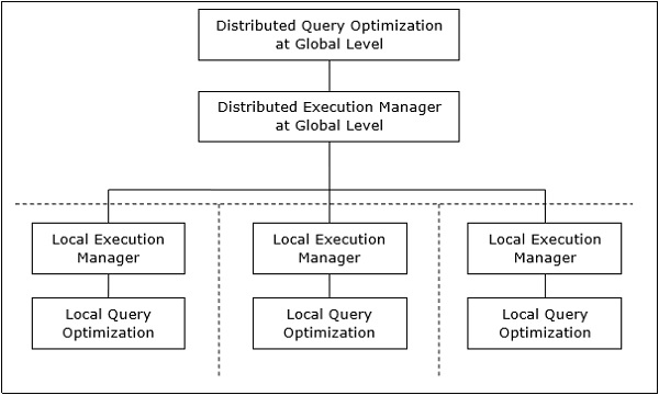
Mapping Global Queries into Local Queries
The process of mapping global queries to local ones can be realized as follows −
The tables required in a global query have fragments distributed across multiple sites. The local databases have information only about local data. The controlling site uses the global data dictionary to gather information about the distribution and reconstructs the global view from the fragments.
If there is no replication, the global optimizer runs local queries at the sites where the fragments are stored. If there is replication, the global optimizer selects the site based upon communication cost, workload, and server speed.
The global optimizer generates a distributed execution plan so that least amount of data transfer occurs across the sites. The plan states the location of the fragments, order in which query steps needs to be executed and the processes involved in transferring intermediate results.
The local queries are optimized by the local database servers. Finally, the local query results are merged together through union operation in case of horizontal fragments and join operation for vertical fragments.
For example, let us consider that the following Project schema is horizontally fragmented according to City, the cities being New Delhi, Kolkata and Hyderabad.
PROJECT
| PId | City | Department | Status |
Suppose there is a query to retrieve details of all projects whose status is Ongoing.
The global query will be &inus;
$$\sigma_{status} = {\small "ongoing"}^{(PROJECT)}$$
Query in New Delhis server will be −
$$\sigma_{status} = {\small "ongoing"}^{({NewD}_-{PROJECT})}$$
Query in Kolkatas server will be −
$$\sigma_{status} = {\small "ongoing"}^{({Kol}_-{PROJECT})}$$
Query in Hyderabads server will be −
$$\sigma_{status} = {\small "ongoing"}^{({Hyd}_-{PROJECT})}$$
In order to get the overall result, we need to union the results of the three queries as follows −
$\sigma_{status} = {\small "ongoing"}^{({NewD}_-{PROJECT})} \cup \sigma_{status} = {\small "ongoing"}^{({kol}_-{PROJECT})} \cup \sigma_{status} = {\small "ongoing"}^{({Hyd}_-{PROJECT})}$
Distributed Query Optimization
Distributed query optimization requires evaluation of a large number of query trees each of which produce the required results of a query. This is primarily due to the presence of large amount of replicated and fragmented data. Hence, the target is to find an optimal solution instead of the best solution.
The main issues for distributed query optimization are −
- Optimal utilization of resources in the distributed system.
- Query trading.
- Reduction of solution space of the query.
Optimal Utilization of Resources in the Distributed System
A distributed system has a number of database servers in the various sites to perform the operations pertaining to a query. Following are the approaches for optimal resource utilization −
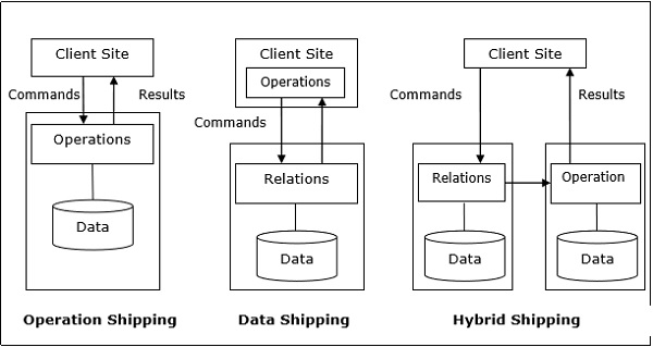
Operation Shipping − In operation shipping, the operation is run at the site where the data is stored and not at the client site. The results are then transferred to the client site. This is appropriate for operations where the operands are available at the same site. Example: Select and Project operations.
Data Shipping − In data shipping, the data fragments are transferred to the database server, where the operations are executed. This is used in operations where the operands are distributed at different sites. This is also appropriate in systems where the communication costs are low, and local processors are much slower than the client server.
Hybrid Shipping − This is a combination of data and operation shipping. Here, data fragments are transferred to the high-speed processors, where the operation runs. The results are then sent to the client site.
Query Trading
In query trading algorithm for distributed database systems, the controlling/client site for a distributed query is called the buyer and the sites where the local queries execute are called sellers. The buyer formulates a number of alternatives for choosing sellers and for reconstructing the global results. The target of the buyer is to achieve the optimal cost.
The algorithm starts with the buyer assigning sub-queries to the seller sites. The optimal plan is created from local optimized query plans proposed by the sellers combined with the communication cost for reconstructing the final result. Once the global optimal plan is formulated, the query is executed.
Reduction of Solution Space of the Query
Optimal solution generally involves reduction of solution space so that the cost of query and data transfer is reduced. This can be achieved through a set of heuristic rules, just as heuristics in centralized systems.
Following are some of the rules −
Perform selection and projection operations as early as possible. This reduces the data flow over communication network.
Simplify operations on horizontal fragments by eliminating selection conditions which are not relevant to a particular site.
In case of join and union operations comprising of fragments located in multiple sites, transfer fragmented data to the site where most of the data is present and perform operation there.
Use semi-join operation to qualify tuples that are to be joined. This reduces the amount of data transfer which in turn reduces communication cost.
Merge the common leaves and sub-trees in a distributed query tree.
DDBMS - Transaction Processing Systems
This chapter discusses the various aspects of transaction processing. Well also study the low level tasks included in a transaction, the transaction states and properties of a transaction. In the last portion, we will look over schedules and serializability of schedules.
Transactions
A transaction is a program including a collection of database operations, executed as a logical unit of data processing. The operations performed in a transaction include one or more of database operations like insert, delete, update or retrieve data. It is an atomic process that is either performed into completion entirely or is not performed at all. A transaction involving only data retrieval without any data update is called read-only transaction.
Each high level operation can be divided into a number of low level tasks or operations. For example, a data update operation can be divided into three tasks −
read_item() − reads data item from storage to main memory.
modify_item() − change value of item in the main memory.
write_item() − write the modified value from main memory to storage.
Database access is restricted to read_item() and write_item() operations. Likewise, for all transactions, read and write forms the basic database operations.
Transaction Operations
The low level operations performed in a transaction are −
begin_transaction − A marker that specifies start of transaction execution.
read_item or write_item − Database operations that may be interleaved with main memory operations as a part of transaction.
end_transaction − A marker that specifies end of transaction.
commit − A signal to specify that the transaction has been successfully completed in its entirety and will not be undone.
rollback − A signal to specify that the transaction has been unsuccessful and so all temporary changes in the database are undone. A committed transaction cannot be rolled back.
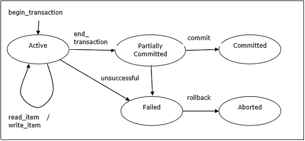
Transaction States
A transaction may go through a subset of five states, active, partially committed, committed, failed and aborted.
Active − The initial state where the transaction enters is the active state. The transaction remains in this state while it is executing read, write or other operations.
Partially Committed − The transaction enters this state after the last statement of the transaction has been executed.
Committed − The transaction enters this state after successful completion of the transaction and system checks have issued commit signal.
Failed − The transaction goes from partially committed state or active state to failed state when it is discovered that normal execution can no longer proceed or system checks fail.
Aborted − This is the state after the transaction has been rolled back after failure and the database has been restored to its state that was before the transaction began.
The following state transition diagram depicts the states in the transaction and the low level transaction operations that causes change in states.
Desirable Properties of Transactions
Any transaction must maintain the ACID properties, viz. Atomicity, Consistency, Isolation, and Durability.
Atomicity − This property states that a transaction is an atomic unit of processing, that is, either it is performed in its entirety or not performed at all. No partial update should exist.
Consistency − A transaction should take the database from one consistent state to another consistent state. It should not adversely affect any data item in the database.
Isolation − A transaction should be executed as if it is the only one in the system. There should not be any interference from the other concurrent transactions that are simultaneously running.
Durability − If a committed transaction brings about a change, that change should be durable in the database and not lost in case of any failure.
Schedules and Conflicts
In a system with a number of simultaneous transactions, a schedule is the total order of execution of operations. Given a schedule S comprising of n transactions, say T1, T2, T3..Tn; for any transaction Ti, the operations in Ti must execute as laid down in the schedule S.
Types of Schedules
There are two types of schedules −
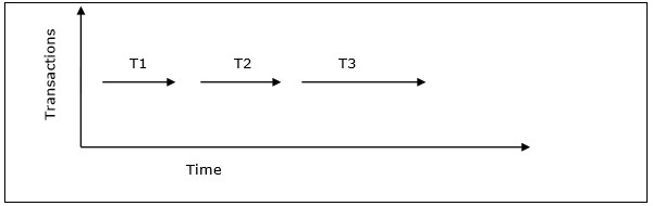
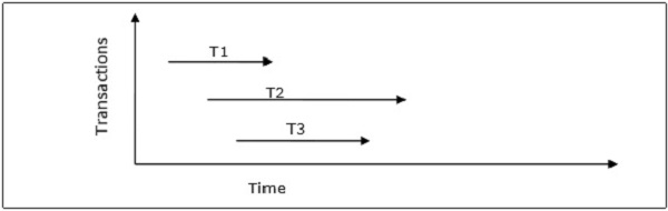
Serial Schedules − In a serial schedule, at any point of time, only one transaction is active, i.e. there is no overlapping of transactions. This is depicted in the following graph −
Parallel Schedules − In parallel schedules, more than one transactions are active simultaneously, i.e. the transactions contain operations that overlap at time. This is depicted in the following graph −
Conflicts in Schedules
In a schedule comprising of multiple transactions, a conflict occurs when two active transactions perform non-compatible operations. Two operations are said to be in conflict, when all of the following three conditions exists simultaneously −
The two operations are parts of different transactions.
Both the operations access the same data item.
At least one of the operations is a write_item() operation, i.e. it tries to modify the data item.
Serializability
A serializable schedule of n transactions is a parallel schedule which is equivalent to a serial schedule comprising of the same n transactions. A serializable schedule contains the correctness of serial schedule while ascertaining better CPU utilization of parallel schedule.
Equivalence of Schedules
Equivalence of two schedules can be of the following types −
Result equivalence − Two schedules producing identical results are said to be result equivalent.
View equivalence − Two schedules that perform similar action in a similar manner are said to be view equivalent.
Conflict equivalence − Two schedules are said to be conflict equivalent if both contain the same set of transactions and has the same order of conflicting pairs of operations.
Distributed DBMS - Controlling Concurrency
Concurrency controlling techniques ensure that multiple transactions are executed simultaneously while maintaining the ACID properties of the transactions and serializability in the schedules.
In this chapter, we will study the various approaches for concurrency control.
Locking Based Concurrency Control Protocols
Locking-based concurrency control protocols use the concept of locking data items. A lock is a variable associated with a data item that determines whether read/write operations can be performed on that data item. Generally, a lock compatibility matrix is used which states whether a data item can be locked by two transactions at the same time.
Locking-based concurrency control systems can use either one-phase or two-phase locking protocols.
One-phase Locking Protocol
In this method, each transaction locks an item before use and releases the lock as soon as it has finished using it. This locking method provides for maximum concurrency but does not always enforce serializability.
Two-phase Locking Protocol
In this method, all locking operations precede the first lock-release or unlock operation. The transaction comprise of two phases. In the first phase, a transaction only acquires all the locks it needs and do not release any lock. This is called the expanding or the growing phase. In the second phase, the transaction releases the locks and cannot request any new locks. This is called the shrinking phase.
Every transaction that follows two-phase locking protocol is guaranteed to be serializable. However, this approach provides low parallelism between two conflicting transactions.
Timestamp Concurrency Control Algorithms
Timestamp-based concurrency control algorithms use a transactions timestamp to coordinate concurrent access to a data item to ensure serializability. A timestamp is a unique identifier given by DBMS to a transaction that represents the transactions start time.
These algorithms ensure that transactions commit in the order dictated by their timestamps. An older transaction should commit before a younger transaction, since the older transaction enters the system before the younger one.
Timestamp-based concurrency control techniques generate serializable schedules such that the equivalent serial schedule is arranged in order of the age of the participating transactions.
Some of timestamp based concurrency control algorithms are −
- Basic timestamp ordering algorithm.
- Conservative timestamp ordering algorithm.
- Multiversion algorithm based upon timestamp ordering.
Timestamp based ordering follow three rules to enforce serializability −
Access Rule − When two transactions try to access the same data item simultaneously, for conflicting operations, priority is given to the older transaction. This causes the younger transaction to wait for the older transaction to commit first.
Late Transaction Rule − If a younger transaction has written a data item, then an older transaction is not allowed to read or write that data item. This rule prevents the older transaction from committing after the younger transaction has already committed.
Younger Transaction Rule − A younger transaction can read or write a data item that has already been written by an older transaction.
Optimistic Concurrency Control Algorithm
In systems with low conflict rates, the task of validating every transaction for serializability may lower performance. In these cases, the test for serializability is postponed to just before commit. Since the conflict rate is low, the probability of aborting transactions which are not serializable is also low. This approach is called optimistic concurrency control technique.
In this approach, a transactions life cycle is divided into the following three phases −
Execution Phase − A transaction fetches data items to memory and performs operations upon them.
Validation Phase − A transaction performs checks to ensure that committing its changes to the database passes serializability test.
Commit Phase − A transaction writes back modified data item in memory to the disk.
This algorithm uses three rules to enforce serializability in validation phase −
Rule 1 − Given two transactions Ti and Tj, if Ti is reading the data item which Tj is writing, then Tis execution phase cannot overlap with Tjs commit phase. Tj can commit only after Ti has finished execution.
Rule 2 − Given two transactions Ti and Tj, if Ti is writing the data item that Tj is reading, then Tis commit phase cannot overlap with Tjs execution phase. Tj can start executing only after Ti has already committed.
Rule 3 − Given two transactions Ti and Tj, if Ti is writing the data item which Tj is also writing, then Tis commit phase cannot overlap with Tjs commit phase. Tj can start to commit only after Ti has already committed.
Concurrency Control in Distributed Systems
In this section, we will see how the above techniques are implemented in a distributed database system.
Distributed Two-phase Locking Algorithm
The basic principle of distributed two-phase locking is same as the basic two-phase locking protocol. However, in a distributed system there are sites designated as lock managers. A lock manager controls lock acquisition requests from transaction monitors. In order to enforce co-ordination between the lock managers in various sites, at least one site is given the authority to see all transactions and detect lock conflicts.
Depending upon the number of sites who can detect lock conflicts, distributed two-phase locking approaches can be of three types −
Centralized two-phase locking − In this approach, one site is designated as the central lock manager. All the sites in the environment know the location of the central lock manager and obtain lock from it during transactions.
Primary copy two-phase locking − In this approach, a number of sites are designated as lock control centers. Each of these sites has the responsibility of managing a defined set of locks. All the sites know which lock control center is responsible for managing lock of which data table/fragment item.
Distributed two-phase locking − In this approach, there are a number of lock managers, where each lock manager controls locks of data items stored at its local site. The location of the lock manager is based upon data distribution and replication.
Distributed Timestamp Concurrency Control
In a centralized system, timestamp of any transaction is determined by the physical clock reading. But, in a distributed system, any sites local physical/logical clock readings cannot be used as global timestamps, since they are not globally unique. So, a timestamp comprises of a combination of site ID and that sites clock reading.
For implementing timestamp ordering algorithms, each site has a scheduler that maintains a separate queue for each transaction manager. During transaction, a transaction manager sends a lock request to the sites scheduler. The scheduler puts the request to the corresponding queue in increasing timestamp order. Requests are processed from the front of the queues in the order of their timestamps, i.e. the oldest first.
Conflict Graphs
Another method is to create conflict graphs. For this transaction classes are defined. A transaction class contains two set of data items called read set and write set. A transaction belongs to a particular class if the transactions read set is a subset of the class read set and the transactions write set is a subset of the class write set. In the read phase, each transaction issues its read requests for the data items in its read set. In the write phase, each transaction issues its write requests.
A conflict graph is created for the classes to which active transactions belong. This contains a set of vertical, horizontal, and diagonal edges. A vertical edge connects two nodes within a class and denotes conflicts within the class. A horizontal edge connects two nodes across two classes and denotes a write-write conflict among different classes. A diagonal edge connects two nodes across two classes and denotes a write-read or a read-write conflict among two classes.
The conflict graphs are analyzed to ascertain whether two transactions within the same class or across two different classes can be run in parallel.
Distributed Optimistic Concurrency Control Algorithm
Distributed optimistic concurrency control algorithm extends optimistic concurrency control algorithm. For this extension, two rules are applied −
Rule 1 − According to this rule, a transaction must be validated locally at all sites when it executes. If a transaction is found to be invalid at any site, it is aborted. Local validation guarantees that the transaction maintains serializability at the sites where it has been executed. After a transaction passes local validation test, it is globally validated.
Rule 2 − According to this rule, after a transaction passes local validation test, it should be globally validated. Global validation ensures that if two conflicting transactions run together at more than one site, they should commit in the same relative order at all the sites they run together. This may require a transaction to wait for the other conflicting transaction, after validation before commit. This requirement makes the algorithm less optimistic since a transaction may not be able to commit as soon as it is validated at a site.
Distributed DBMS - Deadlock Handling
This chapter overviews deadlock handling mechanisms in database systems. Well study the deadlock handling mechanisms in both centralized and distributed database system.
What are Deadlocks?
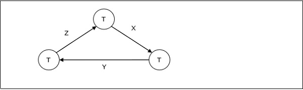
Deadlock is a state of a database system having two or more transactions, when each transaction is waiting for a data item that is being locked by some other transaction. A deadlock can be indicated by a cycle in the wait-for-graph. This is a directed graph in which the vertices denote transactions and the edges denote waits for data items.
For example, in the following wait-for-graph, transaction T1 is waiting for data item X which is locked by T3. T3 is waiting for Y which is locked by T2 and T2 is waiting for Z which is locked by T1. Hence, a waiting cycle is formed, and none of the transactions can proceed executing.
Deadlock Handling in Centralized Systems
There are three classical approaches for deadlock handling, namely −
- Deadlock prevention.
- Deadlock avoidance.
- Deadlock detection and removal.
All of the three approaches can be incorporated in both a centralized and a distributed database system.
Deadlock Prevention
The deadlock prevention approach does not allow any transaction to acquire locks that will lead to deadlocks. The convention is that when more than one transactions request for locking the same data item, only one of them is granted the lock.
One of the most popular deadlock prevention methods is pre-acquisition of all the locks. In this method, a transaction acquires all the locks before starting to execute and retains the locks for the entire duration of transaction. If another transaction needs any of the already acquired locks, it has to wait until all the locks it needs are available. Using this approach, the system is prevented from being deadlocked since none of the waiting transactions are holding any lock.
Deadlock Avoidance
The deadlock avoidance approach handles deadlocks before they occur. It analyzes the transactions and the locks to determine whether or not waiting leads to a deadlock.
The method can be briefly stated as follows. Transactions start executing and request data items that they need to lock. The lock manager checks whether the lock is available. If it is available, the lock manager allocates the data item and the transaction acquires the lock. However, if the item is locked by some other transaction in incompatible mode, the lock manager runs an algorithm to test whether keeping the transaction in waiting state will cause a deadlock or not. Accordingly, the algorithm decides whether the transaction can wait or one of the transactions should be aborted.
There are two algorithms for this purpose, namely wait-die and wound-wait. Let us assume that there are two transactions, T1 and T2, where T1 tries to lock a data item which is already locked by T2. The algorithms are as follows −
Wait-Die − If T1 is older than T2, T1 is allowed to wait. Otherwise, if T1 is younger than T2, T1 is aborted and later restarted.
Wound-Wait − If T1 is older than T2, T2 is aborted and later restarted. Otherwise, if T1 is younger than T2, T1 is allowed to wait.
Deadlock Detection and Removal
The deadlock detection and removal approach runs a deadlock detection algorithm periodically and removes deadlock in case there is one. It does not check for deadlock when a transaction places a request for a lock. When a transaction requests a lock, the lock manager checks whether it is available. If it is available, the transaction is allowed to lock the data item; otherwise the transaction is allowed to wait.
Since there are no precautions while granting lock requests, some of the transactions may be deadlocked. To detect deadlocks, the lock manager periodically checks if the wait-forgraph has cycles. If the system is deadlocked, the lock manager chooses a victim transaction from each cycle. The victim is aborted and rolled back; and then restarted later. Some of the methods used for victim selection are −
- Choose the youngest transaction.
- Choose the transaction with fewest data items.
- Choose the transaction that has performed least number of updates.
- Choose the transaction having least restart overhead.
- Choose the transaction which is common to two or more cycles.
This approach is primarily suited for systems having transactions low and where fast response to lock requests is needed.
Deadlock Handling in Distributed Systems
Transaction processing in a distributed database system is also distributed, i.e. the same transaction may be processing at more than one site. The two main deadlock handling concerns in a distributed database system that are not present in a centralized system are transaction location and transaction control. Once these concerns are addressed, deadlocks are handled through any of deadlock prevention, deadlock avoidance or deadlock detection and removal.
Transaction Location
Transactions in a distributed database system are processed in multiple sites and use data items in multiple sites. The amount of data processing is not uniformly distributed among these sites. The time period of processing also varies. Thus the same transaction may be active at some sites and inactive at others. When two conflicting transactions are located in a site, it may happen that one of them is in inactive state. This condition does not arise in a centralized system. This concern is called transaction location issue.
This concern may be addressed by Daisy Chain model. In this model, a transaction carries certain details when it moves from one site to another. Some of the details are the list of tables required, the list of sites required, the list of visited tables and sites, the list of tables and sites that are yet to be visited and the list of acquired locks with types. After a transaction terminates by either commit or abort, the information should be sent to all the concerned sites.
Transaction Control
Transaction control is concerned with designating and controlling the sites required for processing a transaction in a distributed database system. There are many options regarding the choice of where to process the transaction and how to designate the center of control, like −
- One server may be selected as the center of control.
- The center of control may travel from one server to another.
- The responsibility of controlling may be shared by a number of servers.
Distributed Deadlock Prevention
Just like in centralized deadlock prevention, in distributed deadlock prevention approach, a transaction should acquire all the locks before starting to execute. This prevents deadlocks.
The site where the transaction enters is designated as the controlling site. The controlling site sends messages to the sites where the data items are located to lock the items. Then it waits for confirmation. When all the sites have confirmed that they have locked the data items, transaction starts. If any site or communication link fails, the transaction has to wait until they have been repaired.
Though the implementation is simple, this approach has some drawbacks −
Pre-acquisition of locks requires a long time for communication delays. This increases the time required for transaction.
In case of site or link failure, a transaction has to wait for a long time so that the sites recover. Meanwhile, in the running sites, the items are locked. This may prevent other transactions from executing.
If the controlling site fails, it cannot communicate with the other sites. These sites continue to keep the locked data items in their locked state, thus resulting in blocking.
Distributed Deadlock Avoidance
As in centralized system, distributed deadlock avoidance handles deadlock prior to occurrence. Additionally, in distributed systems, transaction location and transaction control issues needs to be addressed. Due to the distributed nature of the transaction, the following conflicts may occur −
- Conflict between two transactions in the same site.
- Conflict between two transactions in different sites.
In case of conflict, one of the transactions may be aborted or allowed to wait as per distributed wait-die or distributed wound-wait algorithms.
Let us assume that there are two transactions, T1 and T2. T1 arrives at Site P and tries to lock a data item which is already locked by T2 at that site. Hence, there is a conflict at Site P. The algorithms are as follows −
Distributed Wound-Die
If T1 is older than T2, T1 is allowed to wait. T1 can resume execution after Site P receives a message that T2 has either committed or aborted successfully at all sites.
If T1 is younger than T2, T1 is aborted. The concurrency control at Site P sends a message to all sites where T1 has visited to abort T1. The controlling site notifies the user when T1 has been successfully aborted in all the sites.
Distributed Wait-Wait
If T1 is older than T2, T2 needs to be aborted. If T2 is active at Site P, Site P aborts and rolls back T2 and then broadcasts this message to other relevant sites. If T2 has left Site P but is active at Site Q, Site P broadcasts that T2 has been aborted; Site L then aborts and rolls back T2 and sends this message to all sites.
If T1 is younger than T1, T1 is allowed to wait. T1 can resume execution after Site P receives a message that T2 has completed processing.
Distributed Deadlock Detection
Just like centralized deadlock detection approach, deadlocks are allowed to occur and are removed if detected. The system does not perform any checks when a transaction places a lock request. For implementation, global wait-for-graphs are created. Existence of a cycle in the global wait-for-graph indicates deadlocks. However, it is difficult to spot deadlocks since transaction waits for resources across the network.
Alternatively, deadlock detection algorithms can use timers. Each transaction is associated with a timer which is set to a time period in which a transaction is expected to finish. If a transaction does not finish within this time period, the timer goes off, indicating a possible deadlock.
Another tool used for deadlock handling is a deadlock detector. In a centralized system, there is one deadlock detector. In a distributed system, there can be more than one deadlock detectors. A deadlock detector can find deadlocks for the sites under its control. There are three alternatives for deadlock detection in a distributed system, namely.
Centralized Deadlock Detector − One site is designated as the central deadlock detector.
Hierarchical Deadlock Detector − A number of deadlock detectors are arranged in hierarchy.
Distributed Deadlock Detector − All the sites participate in detecting deadlocks and removing them.
Distributed DBMS - Replication Control
This chapter looks into replication control, which is required to maintain consistent data in all sites. We will study the replication control techniques and the algorithms required for replication control.
As discussed earlier, replication is a technique used in distributed databases to store multiple copies of a data table at different sites. The problem with having multiple copies in multiple sites is the overhead of maintaining data consistency, particularly during update operations.
In order to maintain mutually consistent data in all sites, replication control techniques need to be adopted. There are two approaches for replication control, namely −
- Synchronous Replication Control
- Asynchronous Replication Control
Synchronous Replication Control
In synchronous replication approach, the database is synchronized so that all the replications always have the same value. A transaction requesting a data item will have access to the same value in all the sites. To ensure this uniformity, a transaction that updates a data item is expanded so that it makes the update in all the copies of the data item. Generally, two-phase commit protocol is used for the purpose.
For example, let us consider a data table PROJECT(PId, PName, PLocation). We need to run a transaction T1 that updates PLocation to Mumbai, if PLocation is Bombay. If no replications are there, the operations in transaction T1 will be −
Begin T1:
   Update PROJECT Set PLocation = 'Mumbai'
   Where PLocation = 'Bombay';
End T1;
If the data table has two replicas in Site A and Site B, T1 needs to spawn two children T1A and T1B corresponding to the two sites. The expanded transaction T1 will be −
Begin T1:
   Begin T1A :
      Update PROJECT Set PLocation = 'Mumbai'
      Where PLocation = 'Bombay';
   End T1A;

   Begin T2A :
      Update PROJECT Set PLocation = 'Mumbai'
      Where PLocation = 'Bombay';
   End T2A;

End T1;
Asynchronous Replication Control
In asynchronous replication approach, the replicas do not always maintain the same value. One or more replicas may store an outdated value, and a transaction can see the different values. The process of bringing all the replicas to the current value is called synchronization.
A popular method of synchronization is store and forward method. In this method, one site is designated as the primary site and the other sites are secondary sites. The primary site always contains updated values. All the transactions first enter the primary site. These transactions are then queued for application in the secondary sites. The secondary sites are updated using rollout method only when a transaction is scheduled to execute on it.
Replication Control Algorithms
Some of the replication control algorithms are −
- Master-slave replication control algorithm.
- Distributed voting algorithm.
- Majority consensus algorithm.
- Circulating token algorithm.
Master-Slave Replication Control Algorithm
There is one master site and N slave sites. A master algorithm runs at the master site to detect conflicts. A copy of slave algorithm runs at each slave site. The overall algorithm executes in the following two phases −
Transaction acceptance/rejection phase − When a transaction enters the transaction monitor of a slave site, the slave site sends a request to the master site. The master site checks for conflicts. If there arent any conflicts, the master sends an ACK+ message to the slave site which then starts the transaction application phase. Otherwise, the master sends an ACK- message to the slave which then rejects the transaction.
Transaction application phase − Upon entering this phase, the slave site where transaction has entered broadcasts a request to all slaves for executing the transaction. On receiving the requests, the peer slaves execute the transaction and send an ACK to the requesting slave on completion. After the requesting slave has received ACK messages from all its peers, it sends a DONE message to the master site. The master understands that the transaction has been completed and removes it from the pending queue.
Distributed Voting Algorithm
This comprises of N peer sites, all of whom must OK a transaction before it starts executing. Following are the two phases of this algorithm −
Distributed transaction acceptance phase − When a transaction enters the transaction manager of a site, it sends a transaction request to all other sites. On receiving a request, a peer site resolves conflicts using priority based voting rules. If all the peer sites are OK with the transaction, the requesting site starts application phase. If any of the peer sites does not OK a transaction, the requesting site rejects the transaction.
Distributed transaction application phase − Upon entering this phase, the site where the transaction has entered, broadcasts a request to all slaves for executing the transaction. On receiving the requests, the peer slaves execute the transaction and send an ACK message to the requesting slave on completion. After the requesting slave has received ACK messages from all its peers, it lets the transaction manager know that the transaction has been completed.
Majority Consensus Algorithm
This is a variation from the distributed voting algorithm, where a transaction is allowed to execute when a majority of the peers OK a transaction. This is divided into three phases −
Voting phase − When a transaction enters the transaction manager of a site, it sends a transaction request to all other sites. On receiving a request, a peer site tests for conflicts using voting rules and keeps the conflicting transactions, if any, in pending queue. Then, it sends either an OK or a NOT OK message.
Transaction acceptance/rejection phase − If the requesting site receives a majority OK on the transaction, it accepts the transaction and broadcasts ACCEPT to all the sites. Otherwise, it broadcasts REJECT to all the sites and rejects the transaction.
Transaction application phase − When a peer site receives a REJECT message, it removes this transaction from its pending list and reconsiders all deferred transactions. When a peer site receives an ACCEPT message, it applies the transaction and rejects all the deferred transactions in the pending queue which are in conflict with this transaction. It sends an ACK to the requesting slave on completion.
Circulating Token Algorithm
In this approach the transactions in the system are serialized using a circulating token and executed accordingly against every replica of the database. Thus, all the transactions are accepted, i.e. none is rejected. This has two phases −
Transaction serialization phase − In this phase, all transactions are scheduled to run in a serialization order. Each transaction in each site is assigned a unique ticket from a sequential series, indicating the order of transaction. Once a transaction has been assigned a ticket, it is broadcasted to all the sites.
Transaction application phase − When a site receives a transaction along with its ticket, it places the transaction for execution according to its ticket. After the transaction has finished execution, this site broadcasts an appropriate message. A transaction ends when it has completed execution in all the sites.
Distributed DBMS - Failure & Commit
A database management system is susceptible to a number of failures. In this chapter we will study the failure types and commit protocols. In a distributed database system, failures can be broadly categorized into soft failures, hard failures and network failures.
Soft Failure
Soft failure is the type of failure that causes the loss in volatile memory of the computer and not in the persistent storage. Here, the information stored in the non-persistent storage like main memory, buffers, caches or registers, is lost. They are also known as system crash. The various types of soft failures are as follows −
- Operating system failure.
- Main memory crash.
- Transaction failure or abortion.
- System generated error like integer overflow or divide-by-zero error.
- Failure of supporting software.
- Power failure.
Hard Failure
A hard failure is the type of failure that causes loss of data in the persistent or non-volatile storage like disk. Disk failure may cause corruption of data in some disk blocks or failure of the total disk. The causes of a hard failure are −
- Power failure.
- Faults in media.
- Read-write malfunction.
- Corruption of information on the disk.
- Read/write head crash of disk.
Recovery from disk failures can be short, if there is a new, formatted, and ready-to-use disk on reserve. Otherwise, duration includes the time it takes to get a purchase order, buy the disk, and prepare it.
Network Failure
Network failures are prevalent in distributed or network databases. These comprises of the errors induced in the database system due to the distributed nature of the data and transferring data over the network. The causes of network failure are as follows −
- Communication link failure.
- Network congestion.
- Information corruption during transfer.
- Site failures.
- Network partitioning.
Commit Protocols
Any database system should guarantee that the desirable properties of a transaction are maintained even after failures. If a failure occurs during the execution of a transaction, it may happen that all the changes brought about by the transaction are not committed. This makes the database inconsistent. Commit protocols prevent this scenario using either transaction undo (rollback) or transaction redo (roll forward).
Commit Point
The point of time at which the decision is made whether to commit or abort a transaction, is known as commit point. Following are the properties of a commit point.
It is a point of time when the database is consistent.
At this point, the modifications brought about by the database can be seen by the other transactions. All transactions can have a consistent view of the database.
At this point, all the operations of transaction have been successfully executed and their effects have been recorded in transaction log.
At this point, a transaction can be safely undone, if required.
At this point, a transaction releases all the locks held by it.
Transaction Undo
The process of undoing all the changes made to a database by a transaction is called transaction undo or transaction rollback. This is mostly applied in case of soft failure.
Transaction Redo
The process of reapplying the changes made to a database by a transaction is called transaction redo or transaction roll forward. This is mostly applied for recovery from a hard failure.
Transaction Log
A transaction log is a sequential file that keeps track of transaction operations on database items. As the log is sequential in nature, it is processed sequentially either from the beginning or from the end.
Purposes of a transaction log −
- To support commit protocols to commit or support transactions.
- To aid database recovery after failure.
A transaction log is usually kept on the disk, so that it is not affected by soft failures. Additionally, the log is periodically backed up to an archival storage like magnetic tape to protect it from disk failures as well.
Lists in Transaction Logs
The transaction log maintains five types of lists depending upon the status of the transaction. This list aids the recovery manager to ascertain the status of a transaction. The status and the corresponding lists are as follows −
A transaction that has a transaction start record and a transaction commit record, is a committed transaction maintained in commit list.
A transaction that has a transaction start record and a transaction failed record but not a transaction abort record, is a failed transaction maintained in failed list.
A transaction that has a transaction start record and a transaction abort record is an aborted transaction maintained in abort list.
A transaction that has a transaction start record and a transaction before-commit record is a before-commit transaction, i.e. a transaction where all the operations have been executed but not committed maintained in before-commit list.
A transaction that has a transaction start record but no records of before-commit, commit, abort or failed, is an active transaction maintained in active list.
Immediate Update and Deferred Update
Immediate Update and Deferred Update are two methods for maintaining transaction logs.
In immediate update mode, when a transaction executes, the updates made by the transaction are written directly onto the disk. The old values and the updates values are written onto the log before writing to the database in disk. On commit, the changes made to the disk are made permanent. On rollback, changes made by the transaction in the database are discarded and the old values are restored into the database from the old values stored in the log.
In deferred update mode, when a transaction executes, the updates made to the database by the transaction are recorded in the log file. On commit, the changes in the log are written onto the disk. On rollback, the changes in the log are discarded and no changes are applied to the database.
Distributed DBMS - Database Recovery
In order to recuperate from database failure, database management systems resort to a number of recovery management techniques. In this chapter, we will study the different approaches for database recovery.
The typical strategies for database recovery are −
In case of soft failures that result in inconsistency of database, recovery strategy includes transaction undo or rollback. However, sometimes, transaction redo may also be adopted to recover to a consistent state of the transaction.
In case of hard failures resulting in extensive damage to database, recovery strategies encompass restoring a past copy of the database from archival backup. A more current state of the database is obtained through redoing operations of committed transactions from transaction log.
Recovery from Power Failure
Power failure causes loss of information in the non-persistent memory. When power is restored, the operating system and the database management system restart. Recovery manager initiates recovery from the transaction logs.
In case of immediate update mode, the recovery manager takes the following actions −
Transactions which are in active list and failed list are undone and written on the abort list.
Transactions which are in before-commit list are redone.
No action is taken for transactions in commit or abort lists.
In case of deferred update mode, the recovery manager takes the following actions −
Transactions which are in the active list and failed list are written onto the abort list. No undo operations are required since the changes have not been written to the disk yet.
Transactions which are in before-commit list are redone.
No action is taken for transactions in commit or abort lists.
Recovery from Disk Failure
A disk failure or hard crash causes a total database loss. To recover from this hard crash, a new disk is prepared, then the operating system is restored, and finally the database is recovered using the database backup and transaction log. The recovery method is same for both immediate and deferred update modes.
The recovery manager takes the following actions −
The transactions in the commit list and before-commit list are redone and written onto the commit list in the transaction log.
The transactions in the active list and failed list are undone and written onto the abort list in the transaction log.
Checkpointing
Checkpoint is a point of time at which a record is written onto the database from the buffers. As a consequence, in case of a system crash, the recovery manager does not have to redo the transactions that have been committed before checkpoint. Periodical checkpointing shortens the recovery process.
The two types of checkpointing techniques are −
- Consistent checkpointing
- Fuzzy checkpointing
Consistent Checkpointing
Consistent checkpointing creates a consistent image of the database at checkpoint. During recovery, only those transactions which are on the right side of the last checkpoint are undone or redone. The transactions to the left side of the last consistent checkpoint are already committed and neednt be processed again. The actions taken for checkpointing are −
- The active transactions are suspended temporarily.
- All changes in main-memory buffers are written onto the disk.
- A checkpoint record is written in the transaction log.
- The transaction log is written to the disk.
- The suspended transactions are resumed.
If in step 4, the transaction log is archived as well, then this checkpointing aids in recovery from disk failures and power failures, otherwise it aids recovery from only power failures.
Fuzzy Checkpointing
In fuzzy checkpointing, at the time of checkpoint, all the active transactions are written in the log. In case of power failure, the recovery manager processes only those transactions that were active during checkpoint and later. The transactions that have been committed before checkpoint are written to the disk and hence need not be redone.
Example of Checkpointing
Let us consider that in system the time of checkpointing is tcheck and the time of system crash is tfail. Let there be four transactions Ta, Tb, Tc and Td such that −
Ta commits before checkpoint.
Tb starts before checkpoint and commits before system crash.
Tc starts after checkpoint and commits before system crash.
Td starts after checkpoint and was active at the time of system crash.
The situation is depicted in the following diagram −
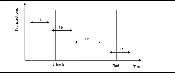
The actions that are taken by the recovery manager are −
- Nothing is done with Ta.
- Transaction redo is performed for Tb and Tc.
- Transaction undo is performed for Td.
Transaction Recovery Using UNDO / REDO
Transaction recovery is done to eliminate the adverse effects of faulty transactions rather than to recover from a failure. Faulty transactions include all transactions that have changed the database into undesired state and the transactions that have used values written by the faulty transactions.
Transaction recovery in these cases is a two-step process −
UNDO all faulty transactions and transactions that may be affected by the faulty transactions.
REDO all transactions that are not faulty but have been undone due to the faulty transactions.
Steps for the UNDO operation are −
If the faulty transaction has done INSERT, the recovery manager deletes the data item(s) inserted.
If the faulty transaction has done DELETE, the recovery manager inserts the deleted data item(s) from the log.
If the faulty transaction has done UPDATE, the recovery manager eliminates the value by writing the before-update value from the log.
Steps for the REDO operation are −
If the transaction has done INSERT, the recovery manager generates an insert from the log.
If the transaction has done DELETE, the recovery manager generates a delete from the log.
If the transaction has done UPDATE, the recovery manager generates an update from the log.
Distributed DBMS - Commit Protocols
In a local database system, for committing a transaction, the transaction manager has to only convey the decision to commit to the recovery manager. However, in a distributed system, the transaction manager should convey the decision to commit to all the servers in the various sites where the transaction is being executed and uniformly enforce the decision. When processing is complete at each site, it reaches the partially committed transaction state and waits for all other transactions to reach their partially committed states. When it receives the message that all the sites are ready to commit, it starts to commit. In a distributed system, either all sites commit or none of them does.
The different distributed commit protocols are −
- One-phase commit
- Two-phase commit
- Three-phase commit
Distributed One-phase Commit
Distributed one-phase commit is the simplest commit protocol. Let us consider that there is a controlling site and a number of slave sites where the transaction is being executed. The steps in distributed commit are −
After each slave has locally completed its transaction, it sends a DONE message to the controlling site.
The slaves wait for Commit or Abort message from the controlling site. This waiting time is called window of vulnerability.
When the controlling site receives DONE message from each slave, it makes a decision to commit or abort. This is called the commit point. Then, it sends this message to all the slaves.
On receiving this message, a slave either commits or aborts and then sends an acknowledgement message to the controlling site.
Distributed Two-phase Commit
Distributed two-phase commit reduces the vulnerability of one-phase commit protocols. The steps performed in the two phases are as follows −
Phase 1: Prepare Phase
After each slave has locally completed its transaction, it sends a DONE message to the controlling site. When the controlling site has received DONE message from all slaves, it sends a Prepare message to the slaves.
The slaves vote on whether they still want to commit or not. If a slave wants to commit, it sends a Ready message.
A slave that does not want to commit sends a Not Ready message. This may happen when the slave has conflicting concurrent transactions or there is a timeout.
Phase 2: Commit/Abort Phase
After the controlling site has received Ready message from all the slaves −
The controlling site sends a Global Commit message to the slaves.
The slaves apply the transaction and send a Commit ACK message to the controlling site.
When the controlling site receives Commit ACK message from all the slaves, it considers the transaction as committed.
After the controlling site has received the first Not Ready message from any slave −
The controlling site sends a Global Abort message to the slaves.
The slaves abort the transaction and send a Abort ACK message to the controlling site.
When the controlling site receives Abort ACK message from all the slaves, it considers the transaction as aborted.
Distributed Three-phase Commit
The steps in distributed three-phase commit are as follows −
Phase 1: Prepare Phase
The steps are same as in distributed two-phase commit.
Phase 2: Prepare to Commit Phase
- The controlling site issues an Enter Prepared State broadcast message.
- The slave sites vote OK in response.
Phase 3: Commit / Abort Phase
The steps are same as two-phase commit except that Commit ACK/Abort ACK message is not required.
DDBMS - Database Security & Cryptography
In this chapter, we will look into the threats that a database system faces and the measures of control. We will also study cryptography as a security tool.
Database Security and Threats
Data security is an imperative aspect of any database system. It is of particular importance in distributed systems because of large number of users, fragmented and replicated data, multiple sites and distributed control.
Threats in a Database
Availability loss − Availability loss refers to non-availability of database objects by legitimate users.
Integrity loss − Integrity loss occurs when unacceptable operations are performed upon the database either accidentally or maliciously. This may happen while creating, inserting, updating or deleting data. It results in corrupted data leading to incorrect decisions.
Confidentiality loss − Confidentiality loss occurs due to unauthorized or unintentional disclosure of confidential information. It may result in illegal actions, security threats and loss in public confidence.
Measures of Control
The measures of control can be broadly divided into the following categories −
Access Control − Access control includes security mechanisms in a database management system to protect against unauthorized access. A user can gain access to the database after clearing the login process through only valid user accounts. Each user account is password protected.
Flow Control − Distributed systems encompass a lot of data flow from one site to another and also within a site. Flow control prevents data from being transferred in such a way that it can be accessed by unauthorized agents. A flow policy lists out the channels through which information can flow. It also defines security classes for data as well as transactions.
Data Encryption − Data encryption refers to coding data when sensitive data is to be communicated over public channels. Even if an unauthorized agent gains access of the data, he cannot understand it since it is in an incomprehensible format.
What is Cryptography?
Cryptography is the science of encoding information before sending via unreliable communication paths so that only an authorized receiver can decode and use it.
The coded message is called cipher text and the original message is called plain text. The process of converting plain text to cipher text by the sender is called encoding or encryption. The process of converting cipher text to plain text by the receiver is called decoding or decryption.
The entire procedure of communicating using cryptography can be illustrated through the following diagram −
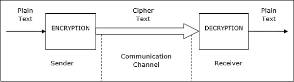
Conventional Encryption Methods
In conventional cryptography, the encryption and decryption is done using the same secret key. Here, the sender encrypts the message with an encryption algorithm using a copy of the secret key. The encrypted message is then send over public communication channels. On receiving the encrypted message, the receiver decrypts it with a corresponding decryption algorithm using the same secret key.
Security in conventional cryptography depends on two factors −
A sound algorithm which is known to all.
A randomly generated, preferably long secret key known only by the sender and the receiver.
The most famous conventional cryptography algorithm is Data Encryption Standard or DES.
The advantage of this method is its easy applicability. However, the greatest problem of conventional cryptography is sharing the secret key between the communicating parties. The ways to send the key are cumbersome and highly susceptible to eavesdropping.
Public Key Cryptography
In contrast to conventional cryptography, public key cryptography uses two different keys, referred to as public key and the private key. Each user generates the pair of public key and private key. The user then puts the public key in an accessible place. When a sender wants to sends a message, he encrypts it using the public key of the receiver. On receiving the encrypted message, the receiver decrypts it using his private key. Since the private key is not known to anyone but the receiver, no other person who receives the message can decrypt it.
The most popular public key cryptography algorithms are RSA algorithm and Diffie Hellman algorithm. This method is very secure to send private messages. However, the problem is, it involves a lot of computations and so proves to be inefficient for long messages.
The solution is to use a combination of conventional and public key cryptography. The secret key is encrypted using public key cryptography before sharing between the communicating parties. Then, the message is send using conventional cryptography with the aid of the shared secret key.
Digital Signatures
A Digital Signature (DS) is an authentication technique based on public key cryptography used in e-commerce applications. It associates a unique mark to an individual within the body of his message. This helps others to authenticate valid senders of messages.
Typically, a users digital signature varies from message to message in order to provide security against counterfeiting. The method is as follows −
The sender takes a message, calculates the message digest of the message and signs it digest with a private key.
The sender then appends the signed digest along with the plaintext message.
The message is sent over communication channel.
The receiver removes the appended signed digest and verifies the digest using the corresponding public key.
The receiver then takes the plaintext message and runs it through the same message digest algorithm.
If the results of step 4 and step 5 match, then the receiver knows that the message has integrity and authentic.
DDBMS - Security in Distributed Databases
A distributed system needs additional security measures than centralized system, since there are many users, diversified data, multiple sites and distributed control. In this chapter, we will look into the various facets of distributed database security.
In distributed communication systems, there are two types of intruders −
Passive eavesdroppers − They monitor the messages and get hold of private information.
Active attackers − They not only monitor the messages but also corrupt data by inserting new data or modifying existing data.
Security measures encompass security in communications, security in data and data auditing.
Communications Security
In a distributed database, a lot of data communication takes place owing to the diversified location of data, users and transactions. So, it demands secure communication between users and databases and between the different database environments.
Security in communication encompasses the following −
Data should not be corrupt during transfer.
The communication channel should be protected against both passive eavesdroppers and active attackers.
In order to achieve the above stated requirements, well-defined security algorithms and protocols should be adopted.
Two popular, consistent technologies for achieving end-to-end secure communications are −
- Secure Socket Layer Protocol or Transport Layer Security Protocol.
- Virtual Private Networks (VPN).
Data Security
In distributed systems, it is imperative to adopt measure to secure data apart from communications. The data security measures are −
Authentication and authorization − These are the access control measures adopted to ensure that only authentic users can use the database. To provide authentication digital certificates are used. Besides, login is restricted through username/password combination.
Data encryption − The two approaches for data encryption in distributed systems are −
Internal to distributed database approach: The user applications encrypt the data and then store the encrypted data in the database. For using the stored data, the applications fetch the encrypted data from the database and then decrypt it.
External to distributed database: The distributed database system has its own encryption capabilities. The user applications store data and retrieve them without realizing that the data is stored in an encrypted form in the database.
Validated input − In this security measure, the user application checks for each input before it can be used for updating the database. An un-validated input can cause a wide range of exploits like buffer overrun, command injection, cross-site scripting and corruption in data.
Data Auditing
A database security system needs to detect and monitor security violations, in order to ascertain the security measures it should adopt. It is often very difficult to detect breach of security at the time of occurrences. One method to identify security violations is to examine audit logs. Audit logs contain information such as −
- Date, time and site of failed access attempts.
- Details of successful access attempts.
- Vital modifications in the database system.
- Access of huge amounts of data, particularly from databases in multiple sites.
All the above information gives an insight of the activities in the database. A periodical analysis of the log helps to identify any unnatural activity along with its site and time of occurrence. This log is ideally stored in a separate server so that it is inaccessible to attackers.
