- Advanced Excel Functions Tutorial
- Advanced Excel Functions - Home
- Compatibility Functions
- Advanced Excel Functions - Cube
- Database Functions
- Date & Time Functions
- Engineering Functions
- Financial Functions
- Information Functions
- Advanced Excel Functions - Logical
- Lookup & Reference Functions
- Math & Trignometric Functions
- Statistical Functions
- Useful Resources
- Quick Guide
- Useful Resources
- Discussion
Lookup and Reference TRANSPOSE Function
Description
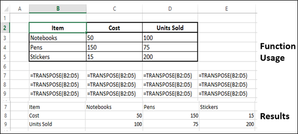
The TRANSPOSE function returns a vertical range of cells as a horizontal range, or vice versa. The TRANSPOSE Function must be entered as an array formula in a range that has the same number of rows and columns, respectively, as the source range has columns and rows.
You can use TRANSPOSE to shift the vertical and horizontal orientation of an array or range on a worksheet.
Syntax
TRANSPOSE (array)
Press CTRL+SHIFT+ENTER after you type the function, as this function returns an array of values, it must be entered as an Array Formula.
Arguments
| Argument | Description | Required/ Optional |
|---|---|---|
| array | An array or range of cells on a worksheet that you want to transpose. The transpose of an array is created by using the first row of the array as the first column of the new array, the second row of the array as the second column of the new array, and so on. |
Required |
Notes
As the result is an Array, you need to input this function as an Array formula −
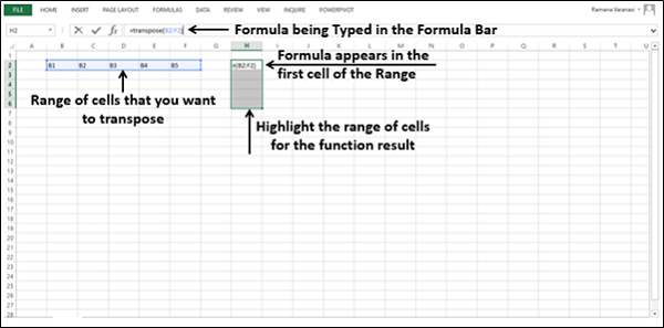
Step 1 − Select the range of cells to be transposed.
Step 2 − Highlight the range of cells for the function result.
Step 3 − Type the function in the formula bar.
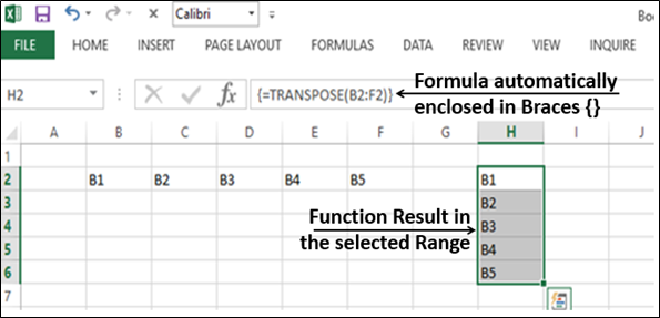
Step 4 − Press CTRL-SHIFT-Enter
Excel surrounds the formula with braces ({ }). You can observe this in the formula bar. It does that automatically, and you cannot enter them yourself. If you do, the formula will not work because Excel treats the braces as text, and it cannot calculate text. Hence, make sure you press Ctrl+Shift+Enter.
Applicability
Excel 2007, Excel 2010, Excel 2013, Excel 2016
Example