- Advanced Excel Functions Tutorial
- Advanced Excel Functions - Home
- Compatibility Functions
- Advanced Excel Functions - Cube
- Database Functions
- Date & Time Functions
- Engineering Functions
- Financial Functions
- Information Functions
- Advanced Excel Functions - Logical
- Lookup & Reference Functions
- Math & Trignometric Functions
- Statistical Functions
- Useful Resources
- Quick Guide
- Useful Resources
- Discussion
GETPIVOTDATA Function
Description
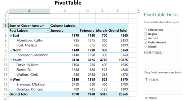
The GETPIVOTDATA function returns data stored in a PivotTable report. You can use it to retrieve summary data from a PivotTable report, provided the summary data is visible in the report.
You can quickly enter a simple GETPIVOTDATA formula by typing = (the equal sign) in the cell you want to return the value to and then clicking the cell in the PivotTable report that contains the data you want to return. Excel then automatically inserts the GETPIVOTDATA function into the active cell.
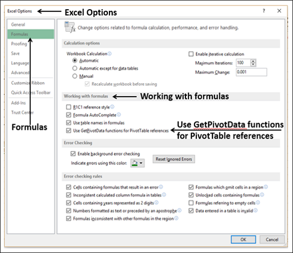
In order to have this quick entry of GETPIVOTDATA function, 'Use GetPivotData functions for PivotTable references' Excel option should be enabled.
Use the following steps −
Step 1 − Click File → Options. The Excel Options Window appears.
Step 2 − Click Formulas in the left pane.
Step 3 − Select 'Use GetPivotData functions for PivotTable references' in the “Working with formulas” section.
Step 4 − Click OK.
Syntax
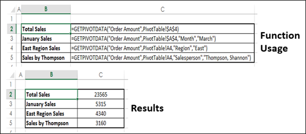
GETPIVOTDATA (data_field, pivot_table, [field1, item1, field2, item2] ...)
Arguments
| Argument | Description | Required/ Optional |
|---|---|---|
| data_field | The name, enclosed in quotation marks, for the data field that contains the data that you want to retrieve. |
Required |
| pivot_table | A reference to any cell, range of cells, or named range of cells in a PivotTable report. This information is used to determine which PivotTable report contains the data that you want to retrieve. |
Required |
| field1, item1, field2, item2 |
1 to 126 pairs of field names and item names that describe the data that you want to retrieve. The pairs can be in any order. Field names and names for items other than dates and numbers are enclosed in quotation marks. For OLAP PivotTable reports, items can contain the source name of the dimension and also the source name of the item. A field and item pair for an OLAP PivotTable might look like this − "[Product]","[Product].[All Products].[Foods].[Baked Goods]" |
Optional |
Notes
Calculated fields or items and custom calculations are included in GETPIVOTDATA calculations.
If pivot_table is a range that includes two or more PivotTable reports, data will be retrieved from whichever report was created most recently in the range.
If the field and item arguments describe a single cell, the value of that cell is returned regardless of whether it is a string, number, error, etc.
If an item contains a date, the value must be expressed as a serial number or populated by using the DATE function so that the value will be retained if the Worksheet is opened in a different location.
For example, an item referring to the date March 5, 1999 could be entered as 36224 or DATE (1999,3,5).
Times can be entered as decimal values or by using the TIME function.
If pivot_table is not a range in which a PivotTable report is found, GETPIVOTDATA returns #REF! error value.
If the arguments do not describe a visible field, or if they include a report filter in which the filtered data is not displayed, GETPIVOTDATA returns the #REF! error value.
Any of the fields specified by the data_field, [field] or [item] arguments are not valid fields within the specified pivot table, GETPIVOTDATA returns the #REF! error value.
Applicability
Excel 2007, Excel 2010, Excel 2013, Excel 2016
Example