- XGBoost - Home
- XGBoost - Overview
- XGBoost - Architecture
- XGBoost - Installation
- XGBoost - Hyper-parameters
- XGBoost - Tuning with Hyper-parameters
- XGBoost - Using DMatrix
- XGBoost - Classification
- XGBoost - Regressor
- XGBoost - Regularization
- XGBoost - Learning to Rank
- XGBoost - Over-fitting Control
- XGBoost - Quantile Regression
- XGBoost - Bootstrapping Approach
- XGBoost - Python Implementation
- XGBoost vs Other Boosting Algorithms
- XGBoost Useful Resources
- XGBoost - Quick Guide
- XGBoost - Useful Resources
- XGBoost - Discussion
XGBoost - Quick Guide
XGBoost - Overview
The open-source software package XGBoost (eXtreme Gradient Boosting) is a regularizing gradient boosting framework that can be used with programming languages like as C++, Java, Python, R, Julia, Perl, and Scala. It is compatible with Linux, macOS, and Microsoft Windows. Developing a Scalable, Portable and Distributed Gradient Boosting (GBM, GBRT, GBDT) Library is the project's main objective. Together with the distributed processing frameworks Apache Hadoop, Spark, Flink, and Dask, it operates on a single system.
In the middle of the 2010s, XGBoost became well known and respected as the preferred algorithm for various machine learning competitions.
How XGBoost Works?
XGBoost creates multiple small trees, each of which improves from the errors of the previous ones. It produces highly precise predictions by combining these trees and using sophisticated algorithms. XGBoost's step-by-step learning and improvement process makes it highly effective and successful for a wide range of machine learning tasks.
Key Features
Here are XGBoost's main features, described below −
Fast and efficient XGBoost is really fast. It handles large amounts of data quickly and uses little memory.
Accurate It usually makes excellent predictions. It is frequently used in competitions and real-world applications since it performs many other techniques in detecting patterns in data.
Flexible You can adjust all of the possibilities to make it more effective for your specific problem. It can handle a wide range of data types, including integers and categories.
Regularization XGBoost includes a strategy for preventing over-fitting, which means it keeps the model from becoming extremely complex and only capable of generating predictions on training data while failing on new data.
XGBoost History
In the mid 2010s XGBoost gained popularity and recognition as the algorithm preferred for many machine learning competition winners.
XGBoost or eXtreme Gradient Boosting debuted on March 27, 2014. Tianqi Chen developed the model as part of a research effort for the Distributed (Deep) Machine Learning Community. This progression highlights the model's origins in academic research and its maturation into a popular machine learning tool.
XGBoost comes within the area of gradient boosting frameworks. It is designed specifically for boosted tree algorithms and is well known for its effectiveness and productivity when working with structured or tabular data.
Because of its versatility and high performance XGBoost is widely used in many different kinds of industries. Some of its most common uses are credit scoring and risk assessment in finance, medical diagnostics for disease prediction, and consumer segmentation and predictive analytics.
And its stable release (2.1.1) were launched on 30 July 2024
Advantages of XGBoost
Here are the main advantages of using XGBoost −
Performance XGBoost is well known for delivering excellent outcomes in a variety of machine learning problems. It has been a popular option for winning solutions in Kaggle contests.
Scalability XGBoost can train machine learning models effectively and scalable as well, which makes it a good choice for large datasets.
Adaptability XGBoost is very configurable because of its wide range of hyper-parameters that can be changed for best performance.
Missing Value Handling XGBoost comes with built-in functionality for handling missing values, which makes working with real-world data which frequently has missing values.
Readability XGBoost offers feature significance, which makes it easier to figure out which variables are more important in generating predictions than some machine learning algorithms that can be challenging to understand.
Disadvantages of XGBoost
Below are some drawbacks of XGBoost you should consider while using it −
XGBoost can be very highly computational, mainly when training complex models, so systems with low resources cannot use it.
When trained on short datasets or with an excessive number of trees in the model, XGBoost is more likely to over-fit.
The numerous XGBoost hyper-parameters that can be altered have to be set correctly in order to maximize performance. However, finding out the perfect mix of variables can need some work and understanding.
Because XGBoost can be resource-intensive, particularly if dealing with large datasets, it is not as suitable for systems with less memory.
When to Use XGBoost
Use XGBoost when you have a problem where you have to use data to make accurate predictions. So use XGBoost when you want high accuracy, fast training, and the ability to handle large, complex datasets, missing data, or irregularities. It is especially helpful when other models fail to operate well or when you need flexibility and control over your model's settings.
Use Cases for XGBoost
XGBoost can be used in many areas −
Finance: To predict stock values, detect fraud, and analyze credit risk.
Healthcare: Predicting disease, patient outcomes, or the creation of novel medications.
Marketing: To predict consumer behavior, focus on specific age groups, or enhance advertisements.
Retail: To predict sales, manage stock levels, or provide product suggestions.
Sports analytics: To predict game outcomes or evaluate player performance.
XGBoost - History & Architecture
XGBoost, or Extreme Gradient Boosting is a machine learning method that use a gradient boosting framework. It offers features like regularization to prevent over-fitting, missing data management, and a customizable method that allows users to define their own optimization goals and criteria.
Architecture of XGBoost
The architecture of XGBoost stands out by its scalable and efficient implementation of gradient boosted decision trees. It includes features like regularization to prevent over-fitting, missing data management, and a customizable approach that allows users to create their own optimization objectives and criteria. These features contribute to the predictive model's robustness and accuracy.
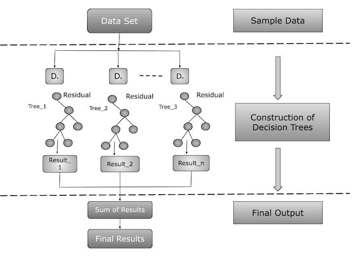
Its architecture can be broadly divided into two main components −
Sequential Learning
XGBoost commonly uses decision trees as its foundational learning. Each subsequent tree is constructed on the previous one's errors, with a focus on misclassified data points. The approach use gradient descent to find the optimal weights for each tree while minimizing the loss function.
Ensemble
XGBoost generates an ensemble of decision trees and combines their predictions to improve overall accuracy. The final forecast is a weighted sum of all the trees' predictions and weighted based on performance.
Key Features of XGBoost Architecture
The XGBoost architecture shows its major components and interconnections. Here is an overview of the architecture's features −
Regularization: XGBoost uses regularization techniques to avoid over-fitting.
Parallel Processing: It employs parallel processing to accelerate training.
Flexibility: It can deal with regression and classification challenges.
High Performance: XGBoost has consistently done well in a wide range of machine learning events.
XGBoost Learning Type
XGBoost depends mainly on supervised learning, which involves learning from labeled data. This method requires building the model on a dataset which has both input features and output labels. This training helps the model to understand the relationship between inputs and outputs, allowing it to make predictions or classifications based on previously unknown data.
XGBoost excels at dealing with structured data and is commonly used for regression (predicting continuous values) and classification (predicting discrete labels).
XGBoost Algorithmic Approach
XGBoost's algorithmic foundation is based on tree based techniques, mainly gradient boosting. Gradient boosting is an ensemble technique that creates multiple decision trees in order, with each tree trying to correct any weaknesses of the previous ones. This creates a strong learner from a large number of weak learners, improving the model's overall accuracy and robustness.
XGBoost is known for combining regularization techniques into its gradient boosting framework. Regularization (both L1 and L2) is used to prevent over-fitting and increase the model's adaptability to fresh data. Also, XGBoost optimizes a loss function during the tree building process, which is crucial for effective learning in regression and classification tasks.
XGBoost's effectiveness and popularity in many types of machine learning applications can be given to its combination of supervised learning and a complicated tree based gradient boosting strategy, which is enhanced with regularization methods.
Summary
XGBoost is a powerful machine learning algorithm that improves predictions by generating and combining several decision trees. It became popular in the mid 2010s after winning several competitions. XGBoost works well with structured data can solve regression and classification problems and use regularization methods to avoid over-fitting.
XGBoost - Installation
XGBoost is an improved distributed gradient boosting library that is fast, versatile, and portable. XGBoost can be installed in a variety of ways, depending on the operating system and development environment. The following are the different methods for installing XGBoost.
Using pip (for Python)
The simplest and most common approach to install XGBoost is via pip. So all you have to do is type the following command into your terminal to download and install the library and its dependencies.
pip install xgboost
Output
Here is the process after running the above command on terminal or command prompt −
Collecting xgboost
  Downloading xgboost-1.7.3-py3-none-manylinux2014_x86_64.whl (199.9 MB)
     199.9/199.9 MB 8.4 MB/s eta 0:00:00
Requirement already satisfied: numpy in /usr/local/lib/python3.8/site-packages (from xgboost) (1.21.2)
Installing collected packages: xgboost
Successfully installed xgboost-1.7.3
Using Conda (for Anaconda users)
If you are working with Anaconda or Miniconda then you can install XGBoost with the help of Conda. When you run the below command it will download the required package and dependencies, then install it in your system.
conda install -c conda-forge xgboost
Outut
The terminal output would typically look like this −
(base) $ conda install -c conda-forge xgboost
Collecting package metadata (current_repodata.json): done
Solving environment: done

## Package Plan ##

  environment location: /path/to/conda/environment

  added / updated specs:
    - xgboost

The following packages will be downloaded:

    package                       |            build
    ------------------------------|-----------------
    xgboost-1.7.3                 |   py38h9b699db_0   70.0 MB
    ------------------------------------------------------------
                                           Total:   70.0 MB

Proceed ([y]/n)? y

Downloading and Extracting Packages
xgboost-1.7.3        |  70.0 MB | ########## | 100%
Preparing transaction: done
Verifying transaction: done
Executing transaction: done
Building from Source
If you want the most latest version of XGBoost or want to make changes to your build, you can do this via source. You will have to install git, cmake, and other build tools on your computer.
-
First you have to clone the XGBoost repository −
git clone --recursive https://github.com/dmlc/xgboost
Below is the terminal output −
$ git clone --recursive https://github.com/dmlc/xgboost
Cloning into 'xgboost'...
remote: Enumerating objects: 17723, done.
remote: Counting objects: 100% (17723/17723), done.
remote: Compressing objects: 100% (4181/4181), done.
remote: Total 17723 (delta 12943), reused 16361 (delta 11547), pack-reused 0
Receiving objects: 100% (17723/17723), 28.36 MiB | 4.61 MiB/s, done.
Resolving deltas: 100% (12943/12943), done.
-
After running the above command you have to navigate to the cloned directory −
cd xgboost
-
Now build the project like below −
mkdir build
cd build
cmake ..
make -j4
The terminal output is as follows −
-- The CXX compiler identification is GNU 9.4.0
-- The C compiler identification is GNU 9.4.0
...
-- Configuring done
-- Generating done
-- Build files have been written to: /path/to/xgboost/build
[  1%] Building CXX object CMakeFiles/xgboost.dir/src/learner.cc.o
[  2%] Building CXX object CMakeFiles/xgboost.dir/src/common/host_device_vector.cc.o
...
[100%] Linking CXX executable xgboost
[100%] Built target xgboost
-
And lastly Install the python package −
cd ../python-package
python setup.py install
Here is the output for the above command after installing the package −
running install
running bdist_egg
running egg_info
creating xgboost.egg-info
writing xgboost.egg-info/PKG-INFO
writing dependency_links to xgboost.egg-info/dependency_links.txt
writing requirements to xgboost.egg-info/requires.txt
writing top-level names to xgboost.egg-info/top_level.txt
writing manifest file 'xgboost.egg-info/SOURCES.txt'
reading manifest file 'xgboost.egg-info/SOURCES.txt'
writing manifest file 'xgboost.egg-info/SOURCES.txt'
installing library code to build/bdist.linux-x86_64/egg
running install_lib
creating /usr/local/lib/python3.8/dist-packages/xgboost-1.7.5-py3.8-linux-x86_64.egg
...
byte-compiling /usr/local/lib/python3.8/dist-packages/xgboost/__init__.py to __init__.cpython-38.pyc
running install_scripts
creating /usr/local/bin
...
running install_egg_info
Writing /usr/local/lib/python3.8/dist-packages/xgboost-1.7.5-py3.8.egg-info
Installing for R
If you want to use the R programming language then XGBoost can be installed from the CRAN repository. Use the below command to install it for R programming −
install.packages('catboost', repos = 'https://cloud.r-project.org/', dependencies=TRUE)
So the command will install CatBoost for R programming. Please refer the below output for installation process on terminal −
Installing package into '/home/user/R/x86_64-pc-linux-gnu-library/4.1'
(as 'lib' is unspecified)
trying URL 'https://cloud.r-project.org/src/contrib/xgboost_1.7.5.tar.gz'
Content type 'application/x-gzip' length 2277833 bytes (2.2 MB)
==================================================
downloaded 2.2 MB

* installing *source* package 'xgboost' ...
** package 'xgboost' successfully unpacked and MD5 sums checked
** using staged installation
** libs

*** Installing xgboost
g++ -std=gnu++11 -I"/usr/share/R/include" -DNDEBUG -I../include -I../third_party/dmlc-core/include -I../third_party/rabit/include -I../third_party/xgboost/src -I../third_party/xgboost/src/../include -fpic -O2 -fPIC -c xgboost_R.cc -o xgboost_R.o
...
...
** R
** demo
** inst
** tests
** preparing package for lazy loading
** help
*** installing help indices
*** copying figures
*** copying HTML documentation
** building package indices
** testing if installed package can be loaded
* DONE (xgboost)
XGBoost - Hyperparameters
In this chapter we are going to discuss the subset of hyperparameters needed or commonly used XGBoost algorithm. These parameters have been selected to simplify the process of generating model parameters from data. The required hyperparameters that need to be configured are listed in this chapter category wise. The hyperparameters that are settable and optional.
XGBoost Hyperparameters Categories
The overall hyperparameters have been divided into three main categories by XGBoost creators −
General Parameters
Booster Parameters
Learning Task Parameters
Let us discuss these three categories of Hyperparameters in the below section −
General Parameters
The general parameters define the overall functionality and working of the XGBoost model. Here is the list of parameters comes in this category −
booster [default=gbtree]: This parameter basically selects the type of model to run at each iteration. It gives 2 options - gbtree: tree-based models and gblinear: linear models.
silent [default=0]: It is used to set the model in silent mode. If it is activated and set to 1, means, no running messages will be printed. It is good to keep it 0 because the messages can help in understanding the model.
nthread [default to the maximum number of threads available]: It is mainly used for parallel processing and the number of cores in the system should be entered. If you want to run on all cores so the value will not be entered and the algorithm will detect it automatically.
There are two other parameters that XGBoost automatically sets so you do not need to worry about them.
Booster Parameters
Since there are two types of boosters, Here we will only discuss the tree booster because it is less frequently used than the linear booster and consistently performs better.
| Parameter | Description | Typical Values |
|---|---|---|
| eta | Like the learning speed. Helps control how much the model changes after each step. | 0.01-0.2 |
| min_child_weight | The smallest total weight of all observations required in a tree's node. | Tune with cross-validation |
| max_depth | The deepest level of a tree. Controls overfitting (model being too specific). | 3-10 |
| max_leaf_nodes | The most leaves (end points) a tree can have. | |
| gamma | The smallest amount the loss needs to decrease to split a node. | Tune based on loss function |
| max_delta_step | Limits how much a tree's weight can change. | Usually not needed |
| subsample | The fraction of the data used to grow each tree. | 0.5-1 |
| colsample_bytree | The fraction of columns (features) randomly chosen for each tree. | 0.5-1 |
| colsample_bylevel | The fraction of columns used for each split at every level of the tree. | Usually not used |
| lambda | L2 regularization (like Ridge regression), helps reduce overfitting. | Try to reduce overfitting |
| alpha | L1 regularization (like Lasso regression), useful for models with many features. | Good for high-dimensional data |
| scale_pos_weight | Helps with imbalanced data classes to make the model learn faster. | > 0 (for imbalanced data) |
Learning Task Parameters
The learning task parameters define the goal of optimization and the metric that will be chosen at each step.
objective [default=reg:linear]
It is used to define the loss function to be minimized. And mostly used values are as follows −
binary: logistic - Refers to binary classification, because there are two classifications. It returns the expected probability instead of the actual class.
multi: softmax - It is used for multiclass classification. It returns the expected class instead of the probability. You also need to set the additional option num_class in order to tell the model how many unique classes are there.
multi: softprob - It is a function that is comparable to softmax in that it provides the probabilities for every possible class that a data point can belong to, instead of only the class that is predicted.
eval_metric [ default according to objective ]
Evaluation metrics must be used with the validation data. The default parameters is rmse used for error classification and regression.
The typical values are as follows −
rmse: root mean square error
mae: mean absolute error
logloss: negative log-likelihood
error: Binary classification error rate (0.5 thresholds)
merror: Multiclass classification error rate
mlogloss: Multiclass logloss
auc: Area under the curve
seed [default=0]
It is the random number seed. And it is used for generating reproducible results and also for parameter tuning.
Those of you who never used Scikit-Learn before are unlikely to recognize these parameter names. However, there is a sklearn wrapper for the Python xgboost package called XGBClassifier parameters. It follows the naming convention of the sklearn style. The names of the parameters that will alter are:
eta -> learning_rate
lambda -> reg_lambda
alpha -> reg_alpha
XGBoost - Tuning with Hyperparameters
In this chapter, we will talk about the crucial problem of XGBoost model hyperparameter adjustment. Hyperparameters are specific numbers or weights that control how an algorithm learns. As we have already seen in the previous chapter XGBoost offers a wide range of hyperparameters. By modifying the hyperparameters of XGBoost we are able to maximize its efficiency. XGBoost is known for its ability to automatically tune thousands of learnable parameters in order to find patterns and regularities in the data.
The decision variables selected at each node are the learnable parameters of tree-based models like XGBoost. Large hyperparameters will result from the increased number of design decisions. These are the parameters that the algorithm is trained with and remains fixed.
Hyperparameters in tree-based models include the maximum tree depth, the number of trees to grow, the number of variables to consider when building each tree, the minimum number of leaf samples, and the fraction of observations used to build a tree. But the focus of this chapter is on maximizing XGBoost hyperparameters, the techniques covered here are applicable to any other advanced ML method.
Tuning XGBoost with Hyperparameters
Now we will see how we can tune our XGBoost model with the help of hyperparameters −
1. Import libraries
First you need to import all the necessary libraries as per the below code −
# Import pandas for handling data
import pandas as pd

# Import numpy for scientific calculations
import numpy as np

# Import XGBoost for machine learning
import xgboost as xgb
from sklearn.metrics import accuracy_score

# Import libraries for tuning hyperparameters
from hyperopt import STATUS_OK, Trials, fmin, hp, tpe
2. Read dataset
Now we will read our dataset. Here we are using Wholesale-customers-data.csv dataset.
data = '/Python/Wholesale customers data.csv'

df = pd.read_csv(data)
3. Declare feature vector and target variables
Here we need to declare the feature vector and target variables now −
X = df.drop('Channel', axis=1)

y = df['Channel']
Now let us take a look at feature vector(X) and target variable(y).
X.head()
y.head()
Output
Here is the outcome of the above step −
0    2
1    2
2    2
3    1
4    2
Name: Channel, dtype: int64
We can see that the y label has values as 1 and 2. We will have to convert it into 0 and 1 for further analysis. So we will do it as follows -
# Change labels into binary values

y[y == 2] = 0

y[y == 1] = 1
And again we will check the y label −
# Now again see the y label

y.head()
Here is the outcome of the above section −
0    0
1    0
2    0
3    1
4    0
Name: Channel, dtype: int64
So you can look here that our target variable (y) is converted into 0 and 1.
4. Split data into separate training and test set
Now we are going to split the above data in the separate training and testing sets. Do it as follows −
from sklearn.model_selection import train_test_split

X_train, X_test, y_train, y_test = train_test_split(X, y, test_size = 0.3, random_state = 0)
Bayesian Optimization with HYPEROPT
Bayesian optimization is the process that finds the optimal parameter for a machine learning or deep learning algorithm. Optimization is the process of determining the lowest cost function that results in a model's overall better performance on both the train and test sets.
In this approach, we will train the model with a variety of parameter ranges until we find the best fit. Hyperparameter tuning helps in finding the optimal tuned parameters and returning the best fit model, which is the best approach to follow when building an ML or DL algorithm.
This chapter discusses one of the most precise and successful hyperparameter tuning methods, Bayesian Optimization with HYPEROPT.
What is HYPEROPT ?
HYPEROPT is an advanced Python package that searches over a hyperparameter space of values to find the best options that minimize the loss function.
The Bayesian Optimization approach use Hyperopt to tune the model hyperparameters. Hyperopt is a Python library for tuning model hyperparameters.
Bayesian Optimization Implementation
The optimization process has 4 parts Initialize domain space, Define objective function, Optimization algorithm and Results. So let us discuss these parts one by one here −
1. Initialize domain space
The domain space refers to the input values for which we want to search. Here is the code you can see −
# Set up hyperparameters for tuning using Hyperopt
space = {
    'max_depth': hp.quniform('max_depth', 3, 10, 1),
    'learning_rate': hp.uniform('learning_rate', 0.01, 0.2),
    'n_estimators': hp.quniform('n_estimators', 50, 300, 50),
    'subsample': hp.uniform('subsample', 0.5, 1),
    'colsample_bytree': hp.uniform('colsample_bytree', 0.5, 1),
    'gamma': hp.uniform('gamma', 0, 0.5),
    'lambda': hp.uniform('lambda', 0, 1),
    'alpha': hp.uniform('alpha', 0, 1)
}
2. Define objective function
The objective function is any function that generates a real value that we want to minimize. In this case, we are focusing to reduce the validation error of a ML model with respect to its hyperparameters. If accuracy is truly valuable, we need to maximize it. The code should then return the metric's negative value.
# Define objective function for hyperparameter tuning
def objective(space):
    clf=xgb.XGBClassifier(
                    n_estimators =space['n_estimators'], max_depth = int(space['max_depth']), gamma = space['gamma'],
                    reg_alpha = int(space['reg_alpha']),min_child_weight=int(space['min_child_weight']),
                    colsample_bytree=int(space['colsample_bytree']))

    evaluation = [( X_train, y_train), ( X_test, y_test)]

    clf.fit(X_train, y_train,
            eval_set=evaluation, eval_metric="auc",
            early_stopping_rounds=10,verbose=False)


    pred = clf.predict(X_test)
    accuracy = accuracy_score(y_test, pred>0.5)
    print ("SCORE:", accuracy)
    return {'loss': -accuracy, 'status': STATUS_OK }
3. Optimization algorithm
It is the procedure for building the surrogate objective function and selecting the next values to evaluate.
# Run Hyperopt to find the best hyperparameters
trials = Trials()
best = fmin(
   fn=objective,
   space=space,
   algo=tpe.suggest,
   max_evals=50,
   trials=trials
)
4. Print Results
The results are score or value pairs used by the algorithm to build the model.
# Print the best hyperparameters
print("Best Hyperparameters:", best)
Output
Best Hyperparameters: {'alpha': 0.221612523499914, 'colsample_bytree': 0.7560822278126258, 'gamma': 0.05019667254058424, 'lambda': 0.3047164013099425, 'learning_rate': 0.019578072539274467, 'max_depth': 9.0, 'n_estimators': 150.0, 'subsample': 0.7674996723810256}
XGBoost - Using DMatrix
XGBoost uses a special data structure called DMatrix to store datasets more effectively. Memory and performance are optimized, particularly if large datasets can be handled with.
Importance of DMatrix
Here are some key points where DMatrix is important in XGBoost −
DMatrix easily stores large datasets by reducing the amount of memory needed.
When your data is changed into a DMatrix so XGBoost can automatically create weights and carry out various preprocessing tasks. It even handles values that are missing.
Using DMatrix instead of a standard dataset format speeds up training because XGBoost can access and use the data quickly.
Example of XGBoost using DMatrix
Here is the step by step process of creating XGboost model with the help of DMatrix −
1. Import Libraries
First you need to import the required libraries for the model.
import xgboost as xgb
import pandas as pd
2. Define the dataset
Define the dataset, this can be your CSV data. Here we have used Wholesale-customers-data.csv dataset.
df = pd.read_csv('/Python/Wholesale-customers-data.csv')
3. Separate features
Now we will separate features (X) and target (y) in this step.
# Features (everything except the 'Channel' column)
X = df.drop(columns=['Channel'])
# Target variable (Channel column)
y = df['Channel']
4. Convert into DMatrix
In this stage we will convert the features and target into a DMatrix which is an optimized data structure for XGBoost.
dtrain = xgb.DMatrix(X, label=y)
5. Define Parameters
Below we will define the XGBoost model parameters.
params = {
   # Maximum depth of a tree
   'max_depth': 3,
   # Learning rate
   'eta': 0.1,
   # Objective function for multiclass classification
   'objective': 'multi:softmax',
   # Number of classes
   'num_class': 3
}
6. Train the model
Now we will train the model with the help of the DMatrix.
num_round = 10  # Number of boosting rounds
bst = xgb.train(params, dtrain, num_round)
7. Save the model and Get Predictions
After training, you can save the model. To make predictions we are using the same data as test but you can use new data in real scenarios.
# Save the model here
bst.save_model('xgboost_model.json')

# Make Predictions here
dtest = xgb.DMatrix(X)
predictions = bst.predict(dtest)

# Print predictions
print(predictions)
Output
This output shows the predicted class for every observation as per the features given.
[2. 2. 2. 1. 2. 2. 2. 2. 1. 2. 2. 1. 2. 2. 2. 1. 2. 1. 2. 1. 2. 1. 1. 2.
 2. 2. 1. 1. 2. 1. 1. 1. 1. 1. 1. 2. 1. 2. 2. 1. 1. 1. 2. 2. 2. 2. 2. 2.
 2. 2. 1. 1. 2. 2. 1. 1. 2. 2. 1. 2. 2. 2. 2. 2. 1. 2. 2. 2. 1. 1. 1. 1.
 1. 1. 2. 1. 1. 2. 1. 1. 1. 2. 2. 1. 2. 2. 2. 1. 1. 1. 1. 1. 2. 1. 2. 1.
 2. 1. 1. 1. 2. 2. 2. 1. 1. 1. 2. 2. 2. 2. 1. 2. 1. 1. 1. 1. 1. 1. 1. 1.
 1. 1. 1. 2. 1. 1. 1. 2. 1. 1. 1. 1. 1. 1. 1. 1. 2. 1. 1. 1. 1. 1. 1. 1.
 1. 2. 1. 1. 1. 1. 1. 1. 1. 1. 1. 2. 2. 1. 2. 2. 2. 1. 1. 2. 2. 2. 2. 1.
 1. 1. 2. 2. 2. 2. 1. 2. 1. 1. 1. 1. 1. 2. 2. 1. 1. 1. 1. 2. 2. 2. 1. 1.
 1. 2. 1. 1. 1. 2. 1. 1. 2. 2. 1. 1. 1. 2. 1. 2. 2. 2. 1. 2. 1. 2. 2. 2.
 2. 1. 2. 1. 1. 2. 1. 1. 1. 1. 2. 1. 1. 1. 1. 1. 1. 1. 1. 1. 1. 1. 1. 1.
 1. 1. 1. 1. 2. 2. 1. 1. 1. 1. 1. 2. 1. 1. 1. 1. 1. 1. 1. 1. 1. 1. 1. 1.
 2. 1. 2. 1. 2. 1. 1. 1. 1. 1. 1. 1. 1. 1. 1. 2. 1. 2. 1. 1. 1. 1. 1. 1.
 1. 1. 1. 1. 1. 2. 1. 1. 1. 2. 2. 1. 2. 2. 2. 2. 2. 2. 2. 1. 1. 2. 1. 1.
 2. 1. 1. 2. 1. 1. 1. 2. 1. 1. 1. 1. 1. 1. 1. 1. 1. 1. 1. 2. 1. 2. 1. 2.
 1. 1. 1. 1. 2. 2. 2. 2. 1. 1. 2. 2. 1. 2. 1. 2. 1. 2. 1. 1. 1. 2. 1. 1.
 1. 1. 1. 1. 1. 2. 1. 1. 1. 1. 1. 1. 1. 2. 1. 1. 2. 1. 1. 1. 1. 1. 1. 1.
 1. 1. 1. 1. 1. 1. 1. 1. 1. 1. 1. 1. 2. 1. 1. 1. 1. 1. 1. 1. 1. 1. 1. 2.
 2. 1. 1. 1. 2. 1. 1. 2. 2. 2. 2. 1. 2. 2. 1. 2. 2. 1. 2. 1. 1. 1. 1. 1.
 1. 1. 2. 1. 1. 2. 1. 1.]
XGBoost - Classification
Among the most common uses of XGBoost is classification. It predicts a discrete class label based on the input features. Classification is carried out using the XGBClassifier module, which was created particularly to handle classification tasks.
XGBClassifier Syntax
To improve performance we can adjust the hyperparameters of the XGBClassifier class in XGBoost. The basic syntax for building an XGBoost classifier is shown below −
model = xgb.XGBClassifier(
    objective='multi:softprob',
    num_class=num_classes,
    max_depth=max_depth,
    learning_rate=learning_rate,
    subsample=subsample,
    colsample_bytree=colsample,
    n_estimators=num_estimators
)
Here is the description of the hyperparameters used in the XGBClassifier syntax −
objective='multi:softprob - It is the objective parameter which is optional for multi-class classification and returns a probability score for each class. For binary classification the default value is 'binary:logistic'.
num_class=num_classes - It is needed for multi-class classification tasks and shows the number of classes present in the dataset.
max_depth=max_depth - It is an optional parameter which shows the maximum depth of each decision tree.
learning_rate=learning_rate - It is an optional parameter in which step size shrinkage avoids overfitting.
subsample=subsample - It is an optional parameter showing the fraction of samples used for each tree.
colsample_bytree=colsample - It is an also optional parameter which shows the fraction of features used for each tree.
n_estimators=num_estimators - It is a required parameter which finds the number of boosting iterations and handles the overall complexity of the model.
Example of XGBoost Classification
The Iris dataset is a highly popular dataset in machine learning. It comprises 150 iris flower examples, each with four measurements and three iris flower species need to be categorized.
Let us use the Iris dataset to show classification using the XGBoost library:
   import xgboost as xgb
   from sklearn.datasets import load_iris
   from sklearn.model_selection import train_test_split
   from sklearn.metrics import accuracy_score, classification_report

   # Load the Iris dataset
   data = load_iris()
   X, y = data.data, data.target

   # Split the data into training and test sets
   X_train, X_test, y_train, y_test = train_test_split(X, y, test_size=0.2, random_state=42)

   #Create an XGBoost classifier
   model = xgb.XGBClassifier()

   #Train the model on the training data
   model.fit(X_train, y_train)

   #Make predictions on the test set
   predictions = model.predict(X_test)

   #Calculate accuracy
   accuracy = accuracy_score(y_test, predictions)

   print("Model's Accuracy is:", accuracy)
   print("\nModel's Classification Report is:")
   print(classification_report(y_test, predictions, target_names=data.target_names))
Output
This will lead to the following outcome −
Model's Accuracy is: 1.0

Model's Classification Report is:
              precision    recall  f1-score   support

      setosa       1.00      1.00      1.00        10
  versicolor       1.00      1.00      1.00         9
   virginica       1.00      1.00      1.00        11

    accuracy                           1.00        30
   macro avg       1.00      1.00      1.00        30
weighted avg       1.00      1.00      1.00        30
Summary
XGBoost is a strong tool for machine learning specially for classification tasks. It works well in many situations because it is fast and has features that help prevent overfitting. For example - we used XGBoost to classify iris flowers into their different types, achieving perfect accuracy of 1.0. Its flexibility and efficiency make XGBoost a great choice for many real life classification problems.
XGBoost - Regressor
Regression is a technique used in XGBoost that predicts continuous numerical values. It is common to use the objective variable in predicting sales, real estate prices, and stock values when it shows a continuous output.
- The results of the regression problems can be real or numbers that are continuous. Two common regression algorithms are decision trees and linear regression. Regression evaluation uses several measures like mean-squared error (MSE) and root-mean-square error (RMSE). These are some of the main components of the XGBoost model each one has a key function.
- The term it stands for is RMSE, or square root of mean squared error. However MAE is an absolute total of the differences between the actual and expected values it is not as commonly used as other metrics because of mathematical errors.
XGBoost is a useful tool for building supervised regression models. This statement can be proven by knowing its objective function and base learners.
- The objective function includes a loss function and a regularization term. It explains the difference between actual and expected values, or how much the output of the model differs from the real data.
- The most popular loss functions in XGBoost for regression and binary classification, respectively, are reg:linear and reg:logistics. XGBoost is a technique used in ensemble learning. Ensemble learning requires training and merging individual models to get a single prediction.
Syntax of XGBRegressor
The XGBRegressor in Python is the regression specific version of XGBoost and is used for regression problems where the objective is to predict continuous numerical values.
The basic syntax to build an XGBRegressor module is as follows −
import xgboost as xgb

model = xgb.XGBRegressor(
   objective='reg:squarederror',
   max_depth=max_depth,
   learning_rate=learning_rate,
   subsample=subsample,
   colsample_bytree=colsample,
   n_estimators=num_estimators
)
Parameters
Here are the parameters of the XGBRegressor function −
objective is a must-have parameter that decides the purpose of the model for regression tasks. It is set to reg which means it uses squared loss to calculate errors in regression problems.
max_depth is an optional parameter that shows how deep each decision tree can go. A higher value allows the tree to learn more, but can also lead to over-fitting.
learning_rate is another optional parameter. It controls how much the model learns in each step. A smaller value can prevent over-fitting by slowing down the learning.
subsample is optional and refers to the portion of data that will be used to create each tree. Using less data can make the model more general.
colsample_bytree is also optional and controls how many features (columns) are used to create each tree.
n_estimators is required and it tells the model how many trees to make (boosting rounds). More trees can improve accuracy but also make the model more complex.
Example of XGBRegressor
This code trains a machine learning model which is used to predict housing prices with the help of the XGBoost method. By reading a dataset and dividing it into training and testing sets, it will train the model. In the end the prediction accuracy is evaluated by computing the root mean squared error or RMSE.
Let us evaluate the regression technique using the XGBoost framework on this dataset −
# Required imports
import numpy as np
import pandas as pd
import xgboost as xg
from sklearn.model_selection import train_test_split
from sklearn.metrics import mean_squared_error as MSE

# Loading the data
dataset = pd.read_csv("/Python/Datasets/HousingData.csv")
X, y = dataset.iloc[:, :-1], dataset.iloc[:, -1]

# Splitting the datasets
train_X, test_X, train_y, test_y = train_test_split(X, y, test_size = 0.3, random_state = 123)

# Instantiation
xgb_r = xg.XGBRegressor(objective ='reg:linear', n_estimators = 10, seed = 123)

# Fitting the model
xgb_r.fit(train_X, train_y)

# Predict the model
pred = xgb_r.predict(test_X)

# RMSE Computation
rmse = np.sqrt(MSE(test_y, pred))
print("RMSE : % f" %(rmse))
Output
Here is the output of the above model −
RMSE : 4.963784
Linear base learner
This code uses a linear booster and XGBoost to predict housing prices. A dataset is loaded split into training and testing sets, and then each set is converted into the DMatrix format needed by XGBoost. The prediction accuracy is determined by calculating the root mean squared error or RMSE after model training.
# Required imports
import numpy as np
import pandas as pd
import xgboost as xg
from sklearn.model_selection import train_test_split
from sklearn.metrics import mean_squared_error as MSE

# Loading the data
dataset = pd.read_csv("/Python/Datasets/HousingData.csv")
X, y = dataset.iloc[:, :-1], dataset.iloc[:, -1]

# Splitting the datasets
train_X, test_X, train_y, test_y = train_test_split(X, y,
					test_size = 0.3, random_state = 123)

train_dmatrix = xg.DMatrix(data = train_X, label = train_y)
test_dmatrix = xg.DMatrix(data = test_X, label = test_y)

# Parameter dictionary
param = {"booster":"gblinear", "objective":"reg:linear"}

xgb_r = xg.train(params = param, dtrain = train_dmatrix, num_boost_round = 10)
pred = xgb_r.predict(test_dmatrix)

# RMSE Computation
rmse = np.sqrt(MSE(test_y, pred))
print("RMSE : % f" %(rmse))
Output
Here is the outcome of the following model −
RMSE : 6.101922
Summary
XGBoost is a popular framework for regression problem resolution. It is ideal for regression models that precisely predict continuous numerical values because of its efficient gradient boosting and ability to handle complex datasets. XGBoost is an important tool for machine learning regression analysis because of its continuous growth, which guarantees that it will lead the way in regression procedures.
XGBoost - Regularization
Strong machine learning algorithm called XGBoost offered a range of regularization techniques with that it reduces over-fitting and improve model generalization.
The following are the main regularization methods for XGBoost −
L1 (Lasso) Regularization: Regulated by the alpha hyperparameter
L2 (Ridge) Regularization: The lambda hyperparameter influences it
Early Stopping: This is controlled by the early_stopping_rounds option.
Minimum Child Weight: Needs each leaf node to have a minimum sum of instance weights.
Gamma: Shows the minimum loss decrease needed to split a leaf node.
Regularization helps manage model complexity by applying penalties to the loss function, stopping the model from fitting noise in the training data.
It is important to know and use these regularization methods in order to optimize XGBoost models and improve performance on unknown data.
L1 and L2 Regularization
XGBoost basically supports 2 primary kind of regularization: first is L1 (Lasso) and second is L2 (Ridge).
L1 (Lasso) Regularization
L1 regularization adds the absolute values of the feature weights to the loss function which encourages weak models by pushing some feature weights to exactly zero.
The alpha hyperparameter in XGBoost controls the L1 regularization strength. At higher alpha levels, more feature weights are set to zero resulting in a simpler and easier-to-understand model.
Mathematical Expression:
Penalty = α × ∑ |weights|
L2 (Ridge) Regularization
L2 regularization is used to add the squared values of the feature weights to the loss function.
As compared with L1, L2 regularization does not drive feature weights to zero; but, it supports lower, more evenly distributed feature weights.
The degree of L2 regularization in XGBoost is controlled by the lambda hyperparameter. Higher lambda values are obtained for a more regularized, feature-weighted, and reduced model.
Mathematical Expression:
Penalty = λ × ∑ (weights)2
Regularization Parameters in XGBoost
Here are the list of parameters used in XGBoost −
alpha (L1 regularization term on weights): By regulating the L1 regularization, this promotes sparse data. Greater alpha values drive more weights to zero by increasing the penalty on weights.
lambda (L2 regularization term on weights): Reduces the weights and complexity of the model by controlling the L2 regularization. The model becomes less sensitive to individual features at higher lambda values.
Early Stopping
XGBoost provides early stopping as a regularization strategy in addition to L1 and L2 regularization. By tracking a verification metric at the time of training and stopping the training process when the metric stops improving, early stopping reduces over-fitting.
The number of rounds to wait before quitting XGBoost if no improvement is seen is set by the early_stopping_rounds option.
Early stopping helps to identify the ideal moment at which the model learned significant patterns without becoming overly sensitive to noise.
Tree-Specific Regularization
XGBoost provides tree-specific regularization techniques. The min_child_weight option sets the minimal total of instance weights for each leaf node in the tree. Higher values provide a lower risk to over-fitting, simpler, more generic trees. This controls the trees' depth and complexity.
Another tree-specific regularization option is the gamma parameter, which determines the lowest loss reduction needed to perform a subsequent division on a leaf node. Higher gamma values result in simpler tree designs and more conservative splits.
Importance of Regularization
In XGBoost by fine tuning alpha and lambda you can control the trade-off between model complexity and performance. So below are some important points given which shows why regularization is important −
Prevents Over-fitting: By penalizing complex models, regularization keeps them from fitting too closely to the training set.
Improves Generalization: Regularization makes sure the model performs well when used with new, untested data.
Better Feature Selection: L1 regularization can be used to drive less important feature weights to zero so removing them from the model and making it easier to read.
XGBoost - Learning To Rank
XGBoost is the most common choice for a wide range of LTR applications, like recommender system enhancement, click-through rate prediction, and SEO. In this chapter we will cover a variety of objective functions, lead you through the steps of preparing data, and provide examples of how to train your model.
What is Learning to Rank?
Before we get started, here we will simply explain what ranking is. Ranking is a subset of supervised machine learning. Rather than predicting the outcome of a single data point, it evaluates a series of data points after receiving a set of data points and a query which sets it apart from the more common situations of classification and regression.
Normally, search engines use ranking to identify the most relevant result. It can also be used to suggest things, provide relevant suggestions based on previous purchases, or, as it did for me, identify the horses with the best probability of winning the next race.
There are three objective functions available for ranking with XGBoost: pointwise, pairwise, and listwise. There are benefits and drawbacks to each of these three objective functions, which stand for different methods of determining the rank of an item group. Many sources provide extensive descriptions of them, but we will focus to the main points here.
Pointwise
This technique processes each query document pair independently. All you have to do is give each query-document pair a score and build a model that can predict the relevance score.
Consider the following situation, we have a dataset of query-document pairs, and each pair has a relevance score between 1 and 5. The relevance score for each pair can be predicted by training a regression model.
The pointwise method is a great way to start since, in addition to its ease of use, it is unexpectedly powerful and challenging to overcome. This method can be applied in XGBoost with any of the typical objective functions for regression or classification. Remember to adjust for any imbalances in the dataset labels.
Pairwise
The pairwise approach evaluates pairings of documents and makes a decision to minimize the number of pairs that are out of order. It is used by algorithms like RankNet.
This approach would take a query and two documents at a time and adjust the predicted relevance scores so that the most relevant document has a higher score than the least relevant one.
It considers the question as well as a single document at a time, as compared to the pointwise method. Here, we want to precisely model the relative order of the documents with respect to a query.
XGBoost provides a few objective functions for this strategy −
rank:pairwise: This is the original pairwise loss function (also called RankNet) that combines LambdaRank with MART (Multiple Additive Regression Trees), also known by the name LambdaMART.
rank:ndcg: NDCG stands for Normalized Discounted Cumulative Gain. It is one of the most popular ranking quality metrics in the industry since it takes into consideration both the relative order of documents given a query and the relevance score of each page. This objective function uses an alternative gradient created from the NDCG metric to optimize the model.
rank:map: MAP stands for Mean Average Precision. This shorter ranking quality metric is used when the relevance scores are binary (0 or 1). If MAP serves as the evaluation metric, then this objective function needs to be used in general.
Listwise
Even if XGBoost not uses the listwise technique, it is still necessary to discuss it for completeness. It considers the entire set of documents for a particular query trying to optimize the list's order all at once.
As it analyzes the relative order of all documents, it is an enhancement over the pointwise and pairwise procedures and may give improved results. An example of a listwise loss function is ListMLE.
Cross-validation is a useful technique to identify the ideal objective function for your problem when trying to choose the optimal goal function. Pointwise was completely ineffective.
Learning to Rank with XGBoost
We will look at how to prepare data and build a Learning to Rank (LTR) model using XGBoost which is a powerful machine learning framework. We will be using the MSLR-WEB10K real-world dataset from Microsoft which is popular in the Learning to Rank community. The relevance ratings of the query-document pairs in this dataset show how closely a document matches the user's query.
Step 1: Preparing the Data
Learning to Rank is a strategy used by search engines to rank results based on relevancy. Given in this set are: What is the person trying to find? The user's outcomes were displayed. Also, the relevance score of every document-four being the highest level of relevance-shows its level of relevance compared to the query. The range of scores is 0 to 4.
Before creating the model we have to import some key libraries for data handling −
import pandas as pd
import numpy as np
from sklearn.datasets import load_svmlight_file
These libraries make handling data easily. NumPy is used for numerical computations, and Pandas is used for data manipulation. The vast, multi-feature dataset is loaded in text format using the load_svmlight_file method from sklearn.datasets.
After that we will load our training and validation datasets −
train = load_svmlight_file(str(data_path / '/Python/vali.txt'), query_id=True)
valid = load_svmlight_file(str(data_path / '/Python/test.txt'), query_id=True)
Our model's training and testing data is stored in train and valid here. Three components make up each dataset: a target vector (relevance scores), a feature matrix (representing document qualities), and query IDs (to group documents under the same query).
Now we will unpack these into variables for using them easily −
X_train, y_train, qid_train = train
X_valid, y_valid, qid_valid = valid
Now, X_train and X_valid are the feature matrices, y_train and y_valid are the relevance scores, and qid_train and qid_valid are used to group the documents by query. We can replicate the ranking task using this approach.
Step 2: Training the XGBRanker
In the training process, we build a model to rank documents according to how relevant they are to a query. By importing the XGBoost library, we will first create the XGBRanker class, which is meant to be used for tasks involving learning to rank.
import xgboost as xgb
model = xgb.XGBRanker(tree_method="hist", objective="rank:ndcg")
Here,
The tree_method="hist" is a fast method for generating decision trees.
The objective="rank:ndcg" setting aims to optimize Normalized Discounted Cumulative Gain (NDCG), a statistic commonly used in ranking activities.
Next we will fit the model to the training data −
model.fit(X_train, y_train, qid=qid_train)
In this case, we pass the query IDs (qid_train), the feature matrix (X_train), and the relevance scores (y_train). One important stage in the ranking process is grouping documents that belong to the same query using query IDs.
Step 3: Predicting Relevance Scores
We can use the model to make predictions once it has been trained. It is usually helpful to forecast relevance for a single query at a time for ranking. Suppose for a moment that we want to predict the outcome of the first query in our validation set −
X_query = X_valid[qid_valid == qids[0]]
Here, X_query contains all the documents relevant to the initial query. Now, we can predict their relevance scores by applying −
y_pred = model.predict(X_query)
The calculated scores will show how relevant each document is in relation to the others. By sorting these predictions, the documents can be scored; higher scores show greater relevance.
Step 4: Evaluating the Model with NDCG
We use a metric called Normalized Discounted Cumulative Gain, or NDCG, to evaluate the effectiveness of our ranking system. This statistic evaluates the degree to which the ranking accurately reflects the actual importance of the papers. Here is the NDCG calculating function −
def ndcg(y_score, y_true, k):
   order = np.argsort(y_score)[::-1]
   y_true = np.take(y_true, order[:k])

   gain = 2 ** y_true - 1
   discounts = np.log2(np.arange(len(y_true)) + 2)
   return np.sum(gain / discounts)
By comparing the expected scores (y_score) and real relevance scores (y_true), this function calculates the NDCG. We go through each query in our validation set and calculate the NDCG score −
ndcg_ = list()
qids = np.unique(qid_valid)

for i, qid in enumerate(qids):
   y = y_valid[qid_valid == qid]

   if np.sum(y) == 0:
      continue

   p = model.predict(X_valid[qid_valid == qid])
   idcg = ndcg(y, y, k=10)
   ndcg_.append(ndcg(p, y, k=10) / idcg)
Finally, we calculate each query's mean NDCG score −
np.mean(ndcg_)
So all we have left is a single score that represents the overall performance of our model. A higher NDCG score indicates a higher ranking quality.
XGBoost - Over-fitting Control
XGBoost is capable to handle large data sets and build highly accurate models which makes it strong. Like any other machine learning model, XGBoost is vulnerable to over-fitting.
Because an over-fitted model collects too much information from the training set, which can contain noise and unimportant patterns, it can perform badly on new, unseen data. In this chapter, we will look at the management of over-fitting in XGBoost.
What is over-fitting?
Before we talk about how over-fitting happens in XGBoost and other gradient boosting models, let's first explain what over-fitting is. Over-fitting happens when a machine learning model pays too much attention to details that are specific to the training data. Instead of learning general patterns that work on other data the model focuses only on the special patterns in the training data. This makes it less useful when trying to make predictions on new data.
Why is over-fitting a problem?
Over-fitting is a problem because it limits the model's ability to function well with new data. If the model focuses too much on patterns that are specific to the training set, it will not be able to find patterns that work for additional data. This means the model will not give good results when used on new or different data.
This is an issue because the majority of machine learning models are designed specifically to identify broad patterns that can be applied to a wide range of people. When applied to unobserved data, a model that has over-fit to the training dataset will not be able to generate accurate predictions.
How to detect over-fitting with XGBoost
The good news is that over-fitting of a machine learning model can be easily identified. All you have to do is to determine that your machine learning model is over-fitting makes predictions on a dataset that was not encountered during training.
Your model is probably not over-fit to the training set if it performs well in making predictions on the unknown dataset. It is likely that your model has over-fit to the training data if the predictions it makes on the unknown data are much poorer than the predictions it makes on the training data.
Does XGBoost have an issue with over-fitting?
For the most part, XGBoost models will over-fit to the training set of data. This is particularly common when developing a complex model with multiple deep trees, or when training an XGBoost model on a limited training dataset.
Compared to other tree-based models like random forest models, XGBoost models have a higher tendency to over-fit to the dataset they were trained on. In general, random forest models are less sensitive to the selection of hyper-parameters used during training than XGBoost and gradient boosted tree models. This means that in order to evaluate the performance of models with various hyperparameter setups, it is very crucial to carry out hyperparameter optimization and make use of cross validation or a validation dataset.
How to avoid over-fitting with XGBoost
Here are some guidelines you can follow when creating an XGBoost or gradient boosted tree model to prevent over-fitting.
1. Use Fewer Trees
One technique to deal with over-fitting in your XGBoost model is to decrease the number of trees in your model. Large, multi-parameter models generally over-fit more frequently than simple, small models. You can simplify and reduce the probability of over-fitting your model by reducing the number of trees in the model.
2. Use Shallow Trees
One alternative way to simplify an XGBoost model and prevent it from over-fitting is to limit the model to use only shallow trees. Each tree therefore undergoes fewer splits, reducing the complexity of the model.
3. Use a Lower Learning Rate
Reducing the learning rate will also make your XGBoost model less vulnerable to over-fitting. This will serve as a regularization technique to prevent your model from being fixated on a pointless detail.
4. Reduce the Number of Features
Another excellent technique to simplify a machine learning model is to limit the features that it can use. This is another useful way to stop an XGboost model from over-fitting.
5. Use a Large Training Dataset
Your training dataset's size is an important factor that could affect how likely it is that your model will over-fit. Using a larger dataset will reduce the probability of over-fitting in your model. If you find that your XGBoost model is over-fitting and you have access to more training data, try increasing the quantity of data you are using to train your model.
Techniques to Control Over-fitting in XGBoost
In order to prevent over-fitting in XGBoost, we can use several approaches. Let's look at each one here −
Regularization: Regularization is one way to keep the model from becoming excessively complex. The model finds it more difficult to store the data because complexity is penalized.
Early Stopping: If, after a predefined number of cycles, the model's performance on a validation set does not improve, you may stop the training process using a technique called "early stopping". This prevents the model from training for an extended period of time and over-fitting the training set.
Limiting the Depth of Trees: As mentioned before very deep trees capture too much detail, which can lead to over-fitting. The depth of the tree can be restricted to keep the model from being too complex.
Learning Rate (Eta): The learning rate of the model determines how rapidly it learns. A greater learning rate leads to faster learning but the capacity of the model to suddenly change its non-universally distributed learning patterns can result to over-fitting.
XGBoost - Quantile Regression
XGBoost is used to predict one primary value at a time, like the average of all possible outcomes. At times, we try to understand every possibility, including the worst-case and best-case situations. This is how Quantile Regression is used.
This is how quantile loss functions are used to train independent XGBoost models. For example- you can train models for the 0.05, 0.5, and 0.95 quantiles to get the lower and upper bounds of the prediction interval.
Because of quantile regression, we can predict other points in the data, or "quantiles," in addition to the mean (average). As an example: 10th percentile (a poor outcome), 50th percentile (average outcome), and 90th percentile (acceptable outcome).
How does Quantile Regression work in XGBoost?
XGBoost regularly reduces errors by focusing its predictions on average. When we use XGBoost combined with Quantile Regression, we adjust the error measurement. Rather than focusing on total errors, we highlight the gap between specific quantiles and predictions.
In simple terms, using Quantile Regression with XGBoost −
It predicts a value for a given percentile.
For a number of cases, we can calculate possible outcomes (bad, average, and good).
For example, this can be useful when creating strategies for both the best and worst case scenarios when it comes to financial estimates.
Quantile Regression with XGBoost
We will import the required libraries to build quantile regression with the help of XGBoost to produce prediction intervals.
import xgboost as xgb
import numpy as np
import matplotlib.pyplot as plt
For training and testing, targets and features are generated from random distributions with the help of synthetic data.
# Generate synthetic data
np.random.seed(42)
X_train = np.random.rand(100, 10)
y_train = np.random.rand(100)
X_test = np.random.rand(20, 10)
To calculate the gradient and Hessian needed to satisfy the XGBoost regressor's objective, a customized quantile loss function is created. Three different quantiles are used to train the models- 0.05, 0.5 (median), and 0.95. These quantiles relate to the lower, median, and upper boundaries of the prediction interval, respectively. After training, each quantile makes predictions on the test set.
def quantile_loss(quantile_value):
   def loss(true_values, predicted_values):
      error = true_values - predicted_values
      gradient = np.where(error > 0, quantile_value, quantile_value - 1)
      # Hessian is constant
      hessian = np.ones_like(error)
      return gradient, hessian
   return loss

quantile_levels = [0.05, 0.5, 0.95]
regression_models = {}

for quantile in quantile_levels:
   regressor = xgb.XGBRegressor(objective=quantile_loss(quantile))
   regressor.fit(X_train, y_train)
   regression_models[quantile] = regressor

# Predicting quantiles
predictions_05 = regression_models[0.05].predict(X_test)
predictions_50 = regression_models[0.5].predict(X_test)
predictions_95 = regression_models[0.95].predict(X_test)

# Lower and upper bounds
lower_prediction = predictions_05
upper_prediction = predictions_95
median_prediction = predictions_50
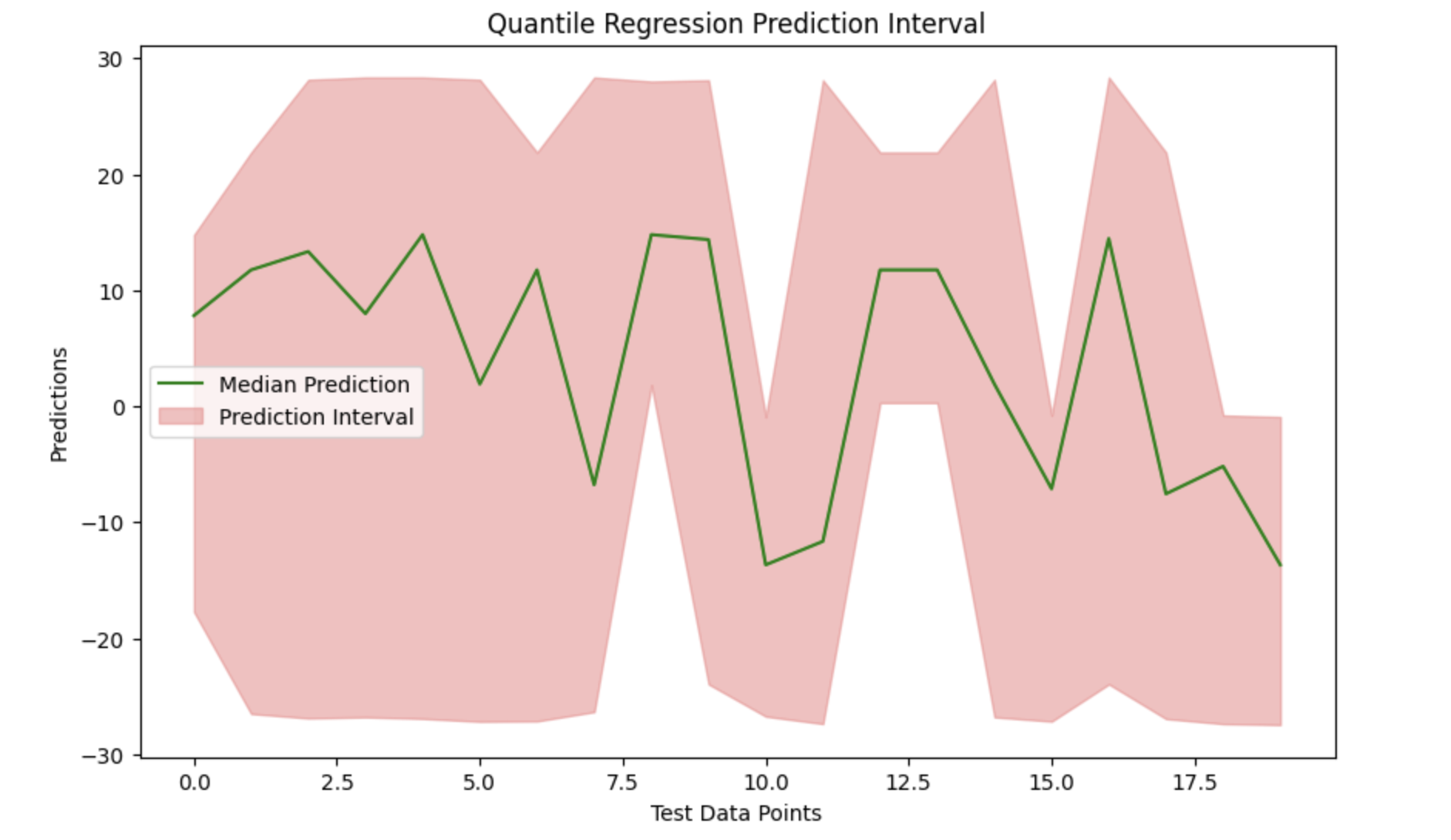
We can see the data and effectively display the prediction interval around the median predictions by plotting the median prediction and filling the gap between the lower and upper boundaries.
# Visualization
plt.figure(figsize=(10, 6))
plt.plot(median_prediction, label='Median Prediction', color='green')
plt.fill_between(range(len(median_prediction)), lower_prediction, upper_prediction, color='lightcoral', alpha=0.5, label='Prediction Interval')
plt.title('Quantile Regression Prediction Interval')
plt.xlabel('Test Data Points')
plt.ylabel('Predictions')
plt.legend()
plt.show()
Output
Here is the outcome of the above model −
XGBoost - Bootstrapping Approach
The bootstrapping method can be combined with replaceable sampling to resample your data and produce many training sets. So, the bootstrapping strategy in XGBoost may be defined as a type of method where we train the model on many random subsets of the data to improve it.
How it works ?
An XGBoost model is trained for each resampled set and predictions are produced for the test data point. The distribution of these predictions provides a rough estimation of the predicted uncertainty.
So the bootstrapping strategy in XGBoost refers to a method of improving the model by training it on many random subsets of the data.
XGBoost generates a huge number of small models each of which is trained on a different portion of the available data. This type of random sampling is referred to as "bootstrapping". XGBoost combines the outputs of these small models and trains on various subsets of the data to produce a single, powerful prediction.
Using different random samples, this strategy attempts to reduce errors and improve model accuracy. It also helps the XGBoost model in avoiding overfitting, which occurs when a model performs well on training data but poorly on new data.
This is similar to how people learn by gaining new experiences.
Apply Bootstrapping to the Model
As we have seen in the bootstrapping method multiple models are trained using resampled versions of the training data, and their predictions are combined. The basic idea is to randomly select data, bootstrap multiple models, and then make predictions on test data that has not been seen before. By averaging the predictions and computing their variability, we can generate confidence intervals that show the degree of uncertainty in our predictions.
So let us see the steps to apply bootstrapping to the XGBoost model −
1. Importing Necessary Libraries and Generating Synthetic Data
First we will load the libraries like XGBoost, NumPy, and Matplotlib for training and analyzing the models. Next, we generate synthetic data to train the models.
# Importing libraries here
import xgboost as xgb
import numpy as np
import matplotlib.pyplot as plt

# Generate random training and testing data
np.random.seed(123)
X_train_data = np.random.rand(150, 8)
y_train_target = np.random.rand(150)

# Generate 30 samples with 8 features for testing
X_test_data = np.random.rand(30, 8)
2. Bootstrapping
Now we will create multiple models by using the above bootstrapping method. Every time we randomly resample the training set, fit an XGBoost model to it and then make predictions about the test set. When we are trying to get a collection of predictions gathered from multiple bootstrapped datasets this method will be repeated multiple times.
# Number of bootstrapped models
n_iterations = 120
# List to store predictions from each model
all_preds = []

for iteration in range(n_iterations):
    # Create a bootstrapped dataset
    sampled_indices = np.random.choice(len(X_train_data), len(X_train_data), replace=True)
    X_resampled_data, y_resampled_target = X_train_data[sampled_indices], y_train_target[sampled_indices]

    # Initialize and train an XGBoost regression model
    xgboost_model = xgb.XGBRegressor()
    xgboost_model.fit(X_resampled_data, y_resampled_target)

    # Make predictions on the test data
    test_predictions = xgboost_model.predict(X_test_data)
    all_preds.append(test_predictions)

# Convert the list of predictions to a NumPy array
all_preds = np.array(all_preds)

# Calculate the mean and standard deviation
avg_preds = np.mean(all_preds, axis=0)
std_dev_preds = np.std(all_preds, axis=0)

# Calculate 95% confidence intervals
lower_confidence_bound = avg_preds - 1.96 * std_dev_preds
upper_confidence_bound = avg_preds + 1.96 * std_dev_preds
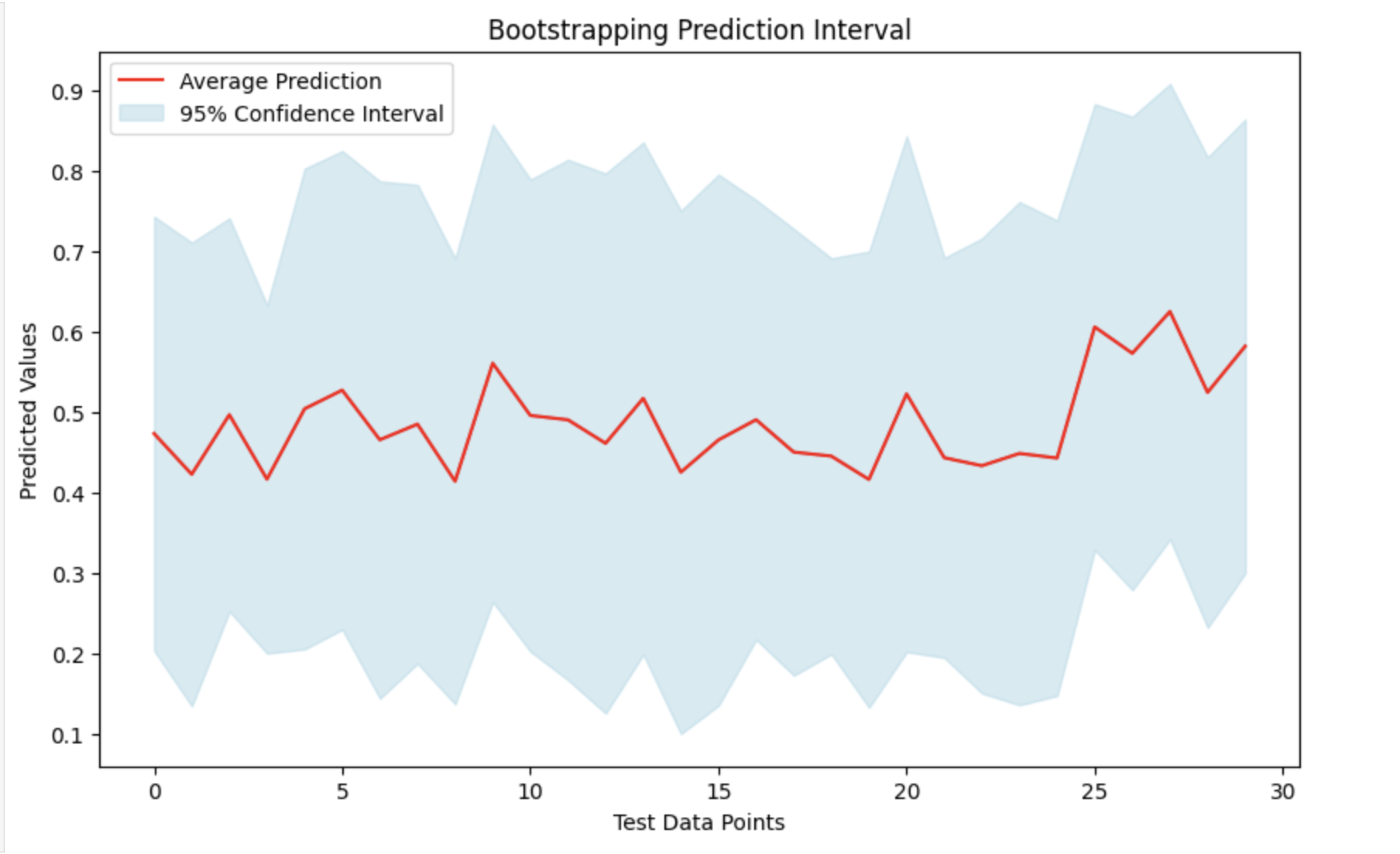
Visualize the Result
By taking the average (mean) of all the predictions and their standard deviations, we can create a prediction interval. This will help us to understand the range in which the actual figures will probably to fall and provides a measure of prediction uncertainty. We can see the findings by plotting the mean forecasts and highlighting the confidence interval around them.
# Visualization of the predictions with confidence intervals
# Set the figure size
plt.figure(figsize=(10, 6))

# Plot the mean predictions
plt.plot(avg_preds, label='Average Prediction', color='red')

# Fill the area between the lower and upper confidence bounds
plt.fill_between(range(len(avg_preds)), lower_confidence_bound, upper_confidence_bound, color='lightblue', alpha=0.5, label='95% Confidence Interval')

# Add title and labels to the plot
plt.title('Bootstrapping Prediction Interval')
plt.xlabel('Test Data Points')
plt.ylabel('Predicted Values')

# Add a legend to describe the plot lines
plt.legend()
# Display the plot
plt.show()
Output
This will produce the following result −
XGBoost - Python Implementation
In this chapter we will use the XGBoost Python module to train an XGBoost model on Titanic data. Our main goal to generate this model is to predict whether a passenger survived by considering variables like age, gender and class. Also we will modify hyper-parameters of our model.
Prerequisites
The following conditions must be met before you can use Python to build an XGBoost model −
Python Environment: It requires Python version 3.6 or later version. You can use a libraries like PyCharm, Visual Studio Code or Jupyter Notebook to write and run your Python code.
Libraries: The Python libraries required for data manipulation, visualization, and machine learning should be installed. The libraries we will be using in our model are scikit-learn, xgboost, matplotlib, pandas, numpy and seaborn.
Dataset: A valid dataset with features and a dependent variable for binary or multi-class classification. The dataset needs to be in a format, like CSV that pandas can load quickly.
Possessing the necessary tools, libraries, dataset, and basic knowledge will help you to use Python for building an XGBoost model.
XGBoost Implementation
Here are the steps you need to follow −
Step 1: Install Needed Libraries
We need some libraries for this implementation so install them with the help of the following commands if you have not already −
# Install necessary libraries
pip install matplotlib
pip install numpy
pip install pandas
pip install scikit-learn
pip install seaborn
pip install xgboost
Step 2: Import Required Libraries
Now you have to import the libraries −
# Here are the imports
import matplotlib.pyplot as plt
import numpy as np
import pandas as pd
import seaborn as sns
import xgboost as xgb
from sklearn.metrics import accuracy_score, confusion_matrix, ConfusionMatrixDisplay
from sklearn.model_selection import GridSearchCV, train_test_split
Step 3: Load the Titanic Dataset
This course will make use of the Titanic dataset which can be downloaded from Kaggle and other sites. So download titanic.csv to get the Titanic dataset. You need to upload a CSV file to your Jupyter Notebook. At this point read the data into a pandas DataFrame −
# Load the dataset
titanic_df = pd.read_csv('/Python/Datasets/titanic.csv')

# Display the first few rows of the dataset
print(titanic_df.head())
Output
This will produce the following result −
   PassengerId  Survived  Pclass  \
0            1         0       3
1            2         1       1
2            3         1       3
3            4         1       1
4            5         0       3

                                                Name     Gender   Age  SibSp  \
0                            Braund, Mr. Owen Harris    male  22.0      1
1  Cumings, Mrs. John Bradley Florence Briggs Th...  female  38.0      1
2                             Heikkinen, Miss. Laina  female  26.0      0
3       Futrelle, Mrs. Jacques Heath (Lily May Peel)  female  35.0      1
4                           Allen, Mr. William Henry    male  35.0      0

   Parch            Ticket     Fare Cabin Embarked
0      0         A/5 21171   7.2500   NaN        S
1      0          PC 17599  71.2833   C85        C
2      0  STON/O2. 3101282   7.9250   NaN        S
3      0            113803  53.1000  C123        S
4      0            373450   8.0500   NaN        S
Step 4: Data Pre-processing
Before we train the model we need the data should be preprocessed. This step includes handling missing data, encoding categorical variables and selecting features. Look for any values that are missing −
# Check for missing values
print(titanic_df.isnull().sum())
Output
This will generate the following result −
PassengerId      0
Survived         0
Pclass           0
Name             0
Gender              0
Age            177
SibSp            0
Parch            0
Ticket           0
Fare             0
Cabin          687
Embarked         2
dtype: int64
Fill in the blanks or remove them −
# Drop rows with missing values
titanic_df = titanic_df.dropna()
Now we will select necessary features and encode categorical variables:
# Select features and target variable
X = titanic_df[['Pclass', 'Gender', 'Age', 'SibSp', 'Parch', 'Fare']]
y = titanic_df['Survived']

# Encode categorical variable 'Gender'
X.loc[:, 'Gender'] = X['Gender'].map({'male': 0, 'female': 1})
Step 5: Train and Evaluate the Model
After separating the data into training and testing sets now we will train the model and evaluate its effectiveness. Here split the data as follows −
# Split data into training and testing sets
X_train, X_test, y_train, y_test = train_test_split(X, y, test_size=0.3, random_state=0)
Next we need to convert the data to DMatrix format for the XGBoost model −
# Convert 'Gender' column to numeric in both training and test sets
X_train['Gender'] = X_train['Gender'].map({'male': 0, 'female': 1})
X_test['Gender'] = X_test['Gender'].map({'male': 0, 'female': 1})

# Ensure there are no missing values and data types are numeric
X_train = X_train.astype(float)
X_test = X_test.astype(float)

# Now convert to DMatrix format
dmatrix_train = xgb.DMatrix(data=X_train, label=y_train)
dmatrix_test = xgb.DMatrix(data=X_test, label=y_test)
Then we will train the model −
# Set learning objective
learning_objective = {'objective': 'binary:logistic'}

# Train the model
model = xgb.train(params=learning_objective, dtrain=dmatrix_train)
After that we have to evaluate the model −
# Make predictions
test_predictions = model.predict(dmatrix_test)
round_test_predictions = [round(p) for p in test_predictions]

# Calculate accuracy
accuracy = accuracy_score(y_test, round_test_predictions)
print(f'Accuracy: {accuracy:.2f}')
Output
This will create the below outcome −
Accuracy: 0.80
Step 6: Hyperparameter Tuning
We will now implement hyper-parameter tuning with GridSearchCV to find the ideal parameters for our XGBoost model. So set up the parameters grid −
# Define the parameter grid
params_grid = {
    'learning_rate': [0.01, 0.05],
    'gamma': [0, 0.01],
    'max_depth': [6, 7],
    'min_child_weight': [1, 2, 3],
    'subsample': [0.6, 0.7],
    'n_estimators': [400, 600, 800],
    'colsample_bytree': [0.7, 0.8],
}
Define and set up the XGBoost classifier and GridSearchCV −
# Define the XGBoost classifier
classifier = xgb.XGBClassifier()

# Set up GridSearchCV
grid_classifier = GridSearchCV(classifier, params_grid, scoring='accuracy', cv=5)
grid_classifier.fit(X_train, y_train)
After determining the most suitable parameters we will evaluate the model:
# Get best parameters
best_parameters = grid_classifier.best_params_
print("Best parameters:", best_parameters)

# Make predictions with the best model
grid_test_preds = grid_classifier.predict(X_test)

# Calculate accuracy
grid_test_accuracy = accuracy_score(y_test, grid_test_preds)
print(f'GridSearchCV Accuracy: {grid_test_accuracy:.2f}')
Output
This will lead to the following outcome −
Best parameters: {'colsample_bytree': 0.7, 'gamma': 0, 'learning_rate': 0.01, 'max_depth': 7, 'min_child_weight': 1, 'n_estimators': 600, 'subsample': 0.7}
GridSearchCV Accuracy: 0.78
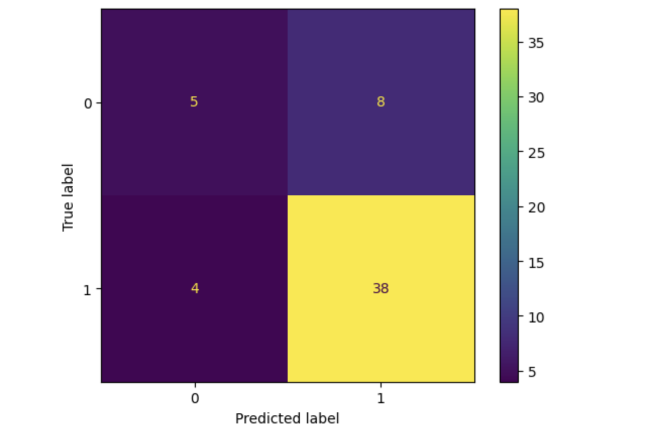
Here we are going to plot the confusion matrix.
# Plot confusion matrix
cm = confusion_matrix(y_test, grid_test_preds)
disp = ConfusionMatrixDisplay(confusion_matrix=cm, display_labels=grid_classifier.classes_)
disp.plot()
plt.show()
Output
This will lead to the following outcome −
Summary
We used the Titanic dataset to explain how to implement an XGBoost model in this chapter. So for improving the model's performance and you can look into alternative datasets.
XGBoost vs Other Boosting Algorithms
Boosting is a popular strategy for machine learning. It combines several weak models to create a stronger model. XGBoost is one of the most widely used boosting algorithms however it is not the only one. In this chapter we will look at how XGBoost compares to other boosting algorithms.
What is XGBoost?
The word XGBoost stands for Extreme Gradient Boosting. It is a machine learning algorithm which is fast, efficient, and accurate. XGBoost is extensively used because it works with a wide range of data formats. It contains unique features that allow it to outperform other algorithms, such as automatically correcting missing data and avoiding over-fitting.
Key Features of XGBoost
Here are some important features of XGBoost you can read while using this method −
Speed: XGBoost is known for its excellent speed. It uses system resources (e.g. memory and CPU) more efficiently than most other algorithms.
Accuracy: XGBoost provides highly accurate predictions because each new model is carefully constructed based on the weaknesses of the previous ones.
Regularization: It is an approach for preventing over-fitting which feature allow the model to perform well with new data.
Parallel computing: XGBoost can operate on several computer cores allowing it to analyze data faster.
Other Boosting Algorithms
There are more boosting algorithms like XGBoost. Let us just discuss them below −
AdaBoost (Adaptive Boosting)
Among the first boosting algorithms was AdaBoost. It combines weak models typically decision trees, by focusing on data points that are challenging to classify. Gradient boosting is used differently by AdaBoost and XGBoost. However it adjusts the weights of incorrectly classified data pieces.
The main difference is that AdaBoost adjusts the data weights, whereas XGBoost focuses on using gradients to fine-tune each model. It may not be as effective with complex data, but it is easier to use than XGBoost.
Gradient Boosting Machine (GBM)
GBM is another prominent boosting algorithm, which is used to serve as the inspiration for XGBoost. It develops models gradually, trying to remove errors from prior models. But GBM is slower than XGBoost due to the lack of parallel processing and regularization features.
Think of XGBoost as a faster and stronger version of GBM. GBM contains fewer built-in features to reduce over-fitting and speed up computations. If you do not need XGBoost's added features or speed you can use GBM instead.
LightGBM
LightGBM is a new boosting algorithm that superior to XGBoost. It takes a different approach by focusing only on significant areas of the data which feature makes it faster and more memory efficient than XGBoost.
The primary difference is that LightGBM typically outperforms XGBoost, especially when working with large datasets. Careful adjustment is likely required to avoid over-fitting, though. You can use LightGBM when working with large datasets when you need results quickly.
CatBoost
CatBoost is another technique that works well with categorical data, which is classified as male or female. CatBoost can automatically convert category data to numerical values but most boosting algorithms, like XGBoost need you to do it.
CatBoost is most effective when your data contains multiple categories which can be difficult for other algorithms. If your data has a high number of categories CatBoost can handle them all automatically by saving your time and effort.
XGBoost vs Other Algorithms
Here we will provide difference between XGBoost and other boosting algorithms in a tabular form −
| Algorithm | Main Strengths | Speed | When to Use |
|---|---|---|---|
| XGBoost | Fast, accurate, prevents over-fitting | Fast | General purpose, large datasets |
| AdaBoost | Simple, focuses on hard-to-classify data | Slow | Simple problems, smaller data |
| GBM | Easy to understand | Slow | If you don't need extra speed |
| LightGBM | Super fast, memory efficient | Very Fast | Very large datasets, speed matters |
| CatBoost | Handles categorical data well | Fast | Datasets with many categories |
