XGBoost - Bootstrapping Approach

The bootstrapping method can be combined with replaceable sampling to resample your data and produce many training sets. So, the bootstrapping strategy in XGBoost may be defined as a type of method where we train the model on many random subsets of the data to improve it.

How it works ?

An XGBoost model is trained for each resampled set and predictions are produced for the test data point. The distribution of these predictions provides a rough estimation of the predicted uncertainty.

So the bootstrapping strategy in XGBoost refers to a method of improving the model by training it on many random subsets of the data.

XGBoost generates a huge number of small models each of which is trained on a different portion of the available data. This type of random sampling is referred to as "bootstrapping". XGBoost combines the outputs of these small models and trains on various subsets of the data to produce a single, powerful prediction.

Using different random samples, this strategy attempts to reduce errors and improve model accuracy. It also helps the XGBoost model in avoiding overfitting, which occurs when a model performs well on training data but poorly on new data.

This is similar to how people learn by gaining new experiences.

Apply Bootstrapping to the Model

As we have seen in the bootstrapping method multiple models are trained using resampled versions of the training data, and their predictions are combined. The basic idea is to randomly select data, bootstrap multiple models, and then make predictions on test data that has not been seen before. By averaging the predictions and computing their variability, we can generate confidence intervals that show the degree of uncertainty in our predictions.

So let us see the steps to apply bootstrapping to the XGBoost model −

1. Importing Necessary Libraries and Generating Synthetic Data

First we will load the libraries like XGBoost, NumPy, and Matplotlib for training and analyzing the models. Next, we generate synthetic data to train the models.

# Importing libraries here
import xgboost as xgb  
import numpy as np  
import matplotlib.pyplot as plt

# Generate random training and testing data
np.random.seed(123)  
X_train_data = np.random.rand(150, 8)  
y_train_target = np.random.rand(150)  

# Generate 30 samples with 8 features for testing
X_test_data = np.random.rand(30, 8)  

2. Bootstrapping

Now we will create multiple models by using the above bootstrapping method. Every time we randomly resample the training set, fit an XGBoost model to it and then make predictions about the test set. When we are trying to get a collection of predictions gathered from multiple bootstrapped datasets this method will be repeated multiple times.

# Number of bootstrapped models
n_iterations = 120  
# List to store predictions from each model
all_preds = []  

for iteration in range(n_iterations):
    # Create a bootstrapped dataset 
    sampled_indices = np.random.choice(len(X_train_data), len(X_train_data), replace=True)
    X_resampled_data, y_resampled_target = X_train_data[sampled_indices], y_train_target[sampled_indices]
    
    # Initialize and train an XGBoost regression model
    xgboost_model = xgb.XGBRegressor()
    xgboost_model.fit(X_resampled_data, y_resampled_target)
    
    # Make predictions on the test data
    test_predictions = xgboost_model.predict(X_test_data)
    all_preds.append(test_predictions)

# Convert the list of predictions to a NumPy array
all_preds = np.array(all_preds)

# Calculate the mean and standard deviation 
avg_preds = np.mean(all_preds, axis=0)
std_dev_preds = np.std(all_preds, axis=0)

# Calculate 95% confidence intervals 
lower_confidence_bound = avg_preds - 1.96 * std_dev_preds
upper_confidence_bound = avg_preds + 1.96 * std_dev_preds

Visualize the Result

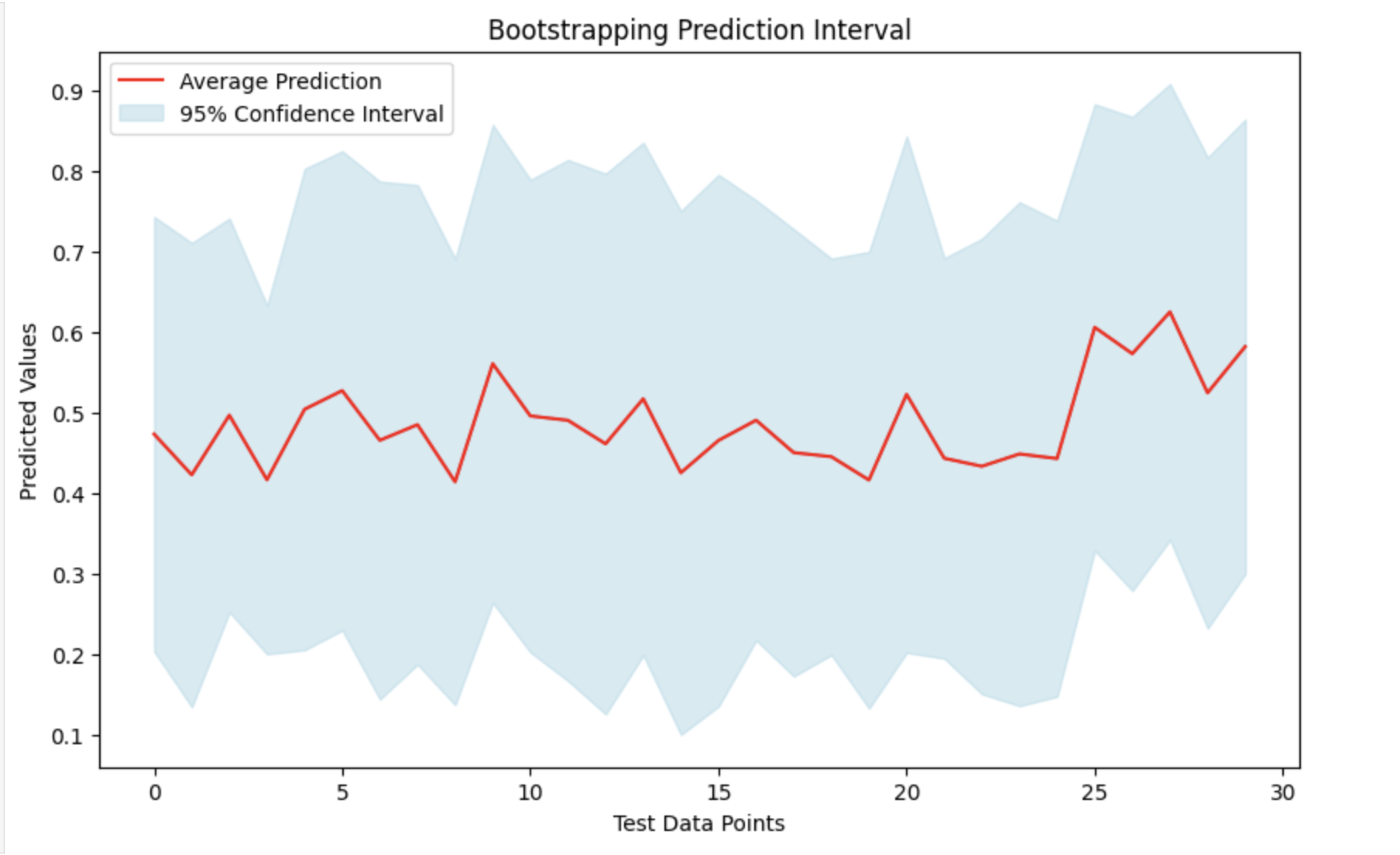
By taking the average (mean) of all the predictions and their standard deviations, we can create a prediction interval. This will help us to understand the range in which the actual figures will probably to fall and provides a measure of prediction uncertainty. We can see the findings by plotting the mean forecasts and highlighting the confidence interval around them.

# Visualization of the predictions with confidence intervals
# Set the figure size
plt.figure(figsize=(10, 6))  

# Plot the mean predictions
plt.plot(avg_preds, label='Average Prediction', color='red')

# Fill the area between the lower and upper confidence bounds
plt.fill_between(range(len(avg_preds)), lower_confidence_bound, upper_confidence_bound, color='lightblue', alpha=0.5, label='95% Confidence Interval')

# Add title and labels to the plot
plt.title('Bootstrapping Prediction Interval') 
plt.xlabel('Test Data Points')  
plt.ylabel('Predicted Values')  

# Add a legend to describe the plot lines
plt.legend()  
# Display the plot
plt.show()  

Output

This will produce the following result −