What is Hierarchical Clustering in R Programming?

Introduction

In the vast area of data analysis and machine learning, hierarchical clustering stands as a powerful technique for grouping individuals or objects based on their similarities. When combined with the versatility and efficiency of R programming language, it becomes an even more invaluable tool for uncovering hidden patterns and structures within large datasets. In this article, we will explore what hierarchical clustering entails, dive into its various types, illustrate with a practical example, and provide a code implementation in R.

Hierarchical Clustering

Hierarchical clustering is an unsupervised learning algorithm that aims to create clusters by iteratively merging or dividing similar entities based on predetermined distance metrics. Unlike other methods like k?means clustering where we need to define the number of desired clusters beforehand, hierarchical clustering constructs a tree?like structure called a dendrogram that can be cut at a certain height to obtain multiple cluster solutions.

Types of Hierarchical Clustering

There are two main approaches when it comes to hierarchical clustering:

• Agglomerative (bottom?up):This method starts by treating everyone as its own cluster and successively merges small clusters together until reaching one big cluster containing all data points. The choice of linkage criterion plays a crucial role here.

• Divisive (top?down): Reverse to agglomerative approach; divisive hierarchical clustering begins with one massive cluster that contains all data points and then recursively divides them into smaller subclusters until achieving individual observations as separate clusters.

R programming to implement the Hierarchical Clustering

The Hierarchical clustering is implemented by calculating the distance with the help of the Manhattan distance.

Algorithm

Step 1:To start with, we first need to load the sample dataset.

Step 2:Before clustering, data preprocessing is necessary. We may need to standardize variables or handle missing values if present.

Step 3:Calculating distances of dissimilarity or distance between observations based on selected metrics such as Euclidean distance or Manhattan distance.

Step 4:Creating Hierarchical Clusters, that we have our distance matrix ready, we can proceed to perform hierarchical clustering using `hclust()` function in R.

Step 5:The resulting object "hc" stores all information required for subsequent steps.

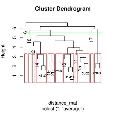
Step 6:Plotting Dendrogram, we can visualize our clusters by plotting dendrograms in R.

Example

library(cluster) 
 
# Create a sample dataset set.seed(123) 
x <- matrix(rnorm(100), ncol = 5) 
 
# Finding distance matrix 
distance_mat <- dist(x, method = 'manhattan') distance_mat 
 
# Fitting Hierarchical Clustering Model 
# to the training dataset set.seed(240) # Setting seed 
Hierar_cl <- hclust(distance_mat, method = "average") 
Hierar_cl 
 
# Plotting dendrogram plot(Hierar_cl) 
 
# Choosing no. of clusters # Cutting tree by height abline(h = 5.5, col = "green") 
 
# Cutting tree by no. of clusters fit <- cutree(Hierar_cl, k = 3 ) fit  table(fit) 
rect.hclust(Hierar_cl, k = 11, border = "red") 

Output

1	2        3        4        5        6        7        8 
2	2.928416                                                                
3	3.820964 4.579451                                                       
4	5.870407 3.963824 6.920070                                              
5	4.712898 3.357644 5.192501 2.041704                                     
6	3.724940 5.188503 2.298511 7.529122 6.906090                            
7	4.378470 3.603915 6.073011 6.448175 6.242628 5.408591                   
8	2.909887 2.270199 5.993941 6.134220 5.627842 5.830570 3.531025          
9	2.545686 4.500523 5.703258 5.466749 3.856739 6.130000 6.203371 4.746715 
10	5.861279 5.127758 9.368977 8.324293 8.236305 8.704556 3.295965 5.013834 
11	6.085281 3.179450 4.827798 5.101238 4.895692 5.436850 2.873268 4.584566 
12	5.590643 2.816420 6.061696 4.307201 3.803264 6.670747 4.914120 4.986817 
13	4.435100 3.563707 6.249931 6.596065 5.579229 5.771611 1.893134 3.980554 
14	6.402935 4.233552 6.619402 4.029210 2.452428 8.633337 5.044223 5.761055 
15	4.785512 2.544131 7.087874 5.618391 5.530404 7.696926 2.610109 3.284796 
16	7.566986 7.161528 6.313095 7.075204 5.756949 6.740845 5.668959 7.578376 
17	6.380095 4.860359 5.530564 7.704619 7.499072 6.327322 3.290148 5.335482 
18	6.818578 4.550758 9.130209 5.378824 5.184404 9.739261 6.419430 4.339261 
19	3.282054 2.655900 3.616115 5.178834 3.243561 4.331110 3.510374 3.815444 
20	3.236401 2.604102 5.008448 5.395216 3.577502 6.633752 5.481153 3.662209 
9	10       11       12       13       14       15       16 
2                                                                          
3                                                                          
4                                                                          
5                                                                          
6                                                                          
7                                                                          
8                                                                          
9                                                                          
10	6.099033                                                                
11	6.734916 5.530202                                                       
12	6.804009 7.368849 4.130914                                              
13	4.591857 3.200043 3.839703 4.870051                                     
14	5.335886 6.919997 4.519932 5.595756 4.300131                            
15	6.393326 3.634753 3.218255 4.662948 4.028726 4.327200                   
16	5.414681 7.171170 5.198525 8.439225 4.010792 3.776011 7.892429          
17	8.925781 6.482177 4.055843 6.170564 5.183282 6.868406 3.874253 8.586946 
18	6.552868 7.159270 5.279163 5.245416 7.472245 6.473367 3.809321 9.815098 
19	3.707689 6.167308 3.286156 3.779404 2.967265 4.302227 5.200031 4.681604 
20	3.297399 6.324931 4.913250 4.907588 4.817754 3.963564 4.663005 6.219969 
         17       18       19 
2                             
3                             
4                             
5 
6
7
8
9
10
11
12
13
14
15
16
17
18 6.804331                  
19 5.625103 6.543116         
20 7.029360 5.821915 2.451658
Call:
hclust(d = distance_mat, method = "average")

Cluster method   : average 
Distance         : manhattan
Number of objects: 20 
  
 [1] 1 1 2 1 1 2 1 1 1 1 1 1 1 1 1 3 2 1 1 1
fit
  1   2  3 
 16   3  1

Conclusion

Hierarchical clustering constitutes a versatile and powerful technique for discovering underlying structures within datasets. By leveraging its practical applications and implementing it through the R programming language, we have now acquired an understanding and hands?on experience with hierarchical clustering. This approach holds immense potential for various domains like customer segmentation, image analysis, and bioinformatics assisting experts in unveiling hidden patterns that help drive informed decision?making processes.