
Article Categories
- All Categories
-
 Data Structure
-
 Networking
-
 RDBMS
RDBMS
-
 Operating System
-
 Java
Java
-
 MS Excel
-
 iOS
iOS
-
 HTML
HTML
-
 CSS
CSS
-
 Android
-
 Python
-
 C Programming
-
 C++
C++
-
 C#
C#
-
 MongoDB
-
 MySQL
MySQL
-
 Javascript
-
 PHP
PHP
-
 Economics & Finance
Simple Linear Regression in Machine Learning
Introduction: Simple Linear Regression
The "Supervised Machine Learning" algorithm of regression is used to forecast continuous features.
The simplest regression procedure, linear regression fits a linear equation or "best fit line" to the observed data in an effort to explain the connection between the dependent variable one and or more independent variables.
There are two versions of linear regression depending on the number of characteristics used as input
Multiple Linear Regression
Simple Linear Regression
In this article, we will be exploring the concept of Simple Linear Regression.
Simple Linear Regression Model
A form of regression method called simple linear regression simulates the relationship between a given independent variable and a dependent variable. A Simple Linear Regression model displays a linear or sloping straight-line relationship.
A straight line can be used in simple linear regression to establish the link between two variables. Finding the slope and intercept, which both define the line and reduce regression errors, is the first step in drawing the line.
One x variable and one y variable make up simple linear regression's most basic version. Because it cannot be predicted by the dependent variable, the x variable is the independent variable. The fact that the y variable is contingent on the prediction we make makes it the dependent variable.
The dependent variable for simple linear regression must have a continuous or real value. However, the independent variable can indeed be assessed on continuous or categorical values.
The two major goals of the simple linear regression algorithm are as follows
Model how the two variables are related. For instance, the connection between income and spending, experience and pay, etc.
Anticipating fresh observations Examples include predicting the weather based on temperature, calculating a company's revenue based on its annual investments, etc.
The equation below can be used to illustrate the Simple Linear Regression model
y= a0+a1x+ ?
Where
The regression line's intercept, denoted by the symbol a0, can be obtained by putting x=0.
The slope of the regression line, or a1, indicates whether the line is rising or falling.
? = The incorrect term.
Python Implementation Of The SLR Algorithm
Here, we are taking a dataset with two variables: experience and income (dependent variable) (Independent variable). The objectives of this issue are -
In order to determine whether these two variables are correlated,
The dataset's best fit line will be found.
How modifying the independent variable affects the dependent variable
To determine which line best represents the relationship between the two variables, we will build a simple linear regression model in this section.
The following actions must be taken in implementing the Simple Linear Regression model in Python.
Step 1: Data Pre-Processing
Data pre-processing is the initial step in the creation of the Simple Linear Regression model. This tutorial already covered it earlier. However, there will be adjustments, as detailed in the following steps -
Prior to importing the dataset, constructing the graphs, and building the Simple Linear Regression model, we will import three crucial libraries.
<div class="code-mirror  language-python" contenteditable="plaintext-only" spellcheck="false" style="outline: none; overflow-wrap: break-word; overflow-y: auto; white-space: pre-wrap;"><span class="token keyword">import</span> numpy <span class="token keyword">as</span> np
<span class="token keyword">import</span> matplotlib<span class="token punctuation">.</span>pyplot <span class="token keyword">as</span> mtplt
<span class="token keyword">import</span> pandas <span class="token keyword">as</span> ps
</div>
The dataset will then be loaded into our code.
data_set= ps.read_csv('Salarynov_Data.csv')
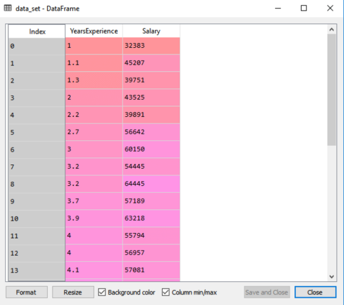
We can access the dataset on our Spyder IDE screen by selecting the variable explorer option by running the code above (ctrl+ENTER).
The dataset, which includes the two variables experience and salary, is displayed in the output.
The dependent and independent variables must then be extracted from the provided dataset. Years of experience are an independent variable, and salary is a dependent variable. The code is as follows
a= data_set.iloc[:, :-1].values
b= data_set.iloc[:, 1].values
Since we want to eliminate the last column from of the dataset, we gave the a variable in the lines of code above a value of -1. We used the number 1 for the b variable because we want to extract the second column because indexing starts at 0.
The training set and test set will then be divided into two groups. We will use 20 observations for the training set and 10 observations for the test set out of the total 30 observations we have. We divide our dataset into training and test sets so that we can use one set to train and the other to test our model.
Step 2. Fitting The Training Set Into The SLR
Fitting our model towards the training dataset is the next step. To do this, we will import the Linear Regression class from the scikit-learn linear model package. Following class import, we will make a regressor object, which is a subclass of the class.
<div class="code-mirror  language-python" contenteditable="plaintext-only" spellcheck="false" style="outline: none; overflow-wrap: break-word; overflow-y: auto; white-space: pre-wrap;"><span class="token keyword">from</span> sklearn<span class="token punctuation">.</span>linear_model <span class="token keyword">import</span> LinearRegressionres
regressor<span class="token operator">=</span> LinearRegressionres<span class="token punctuation">(</span><span class="token punctuation">)</span>
regressor<span class="token punctuation">.</span>fit<span class="token punctuation">(</span>a_train<span class="token punctuation">,</span> b_train<span class="token punctuation">)</span>
</div>
Our training datasets for the dependent and independent variables, x train and y train, have been supplied to the fit() function. So that the model may learn very quickly the correlations between the predictor and target variables, we fitted our regressor object to the training set.
Step 3. Test Result Prediction
Salary is a dependent variable and then an independent one (Experience). As a result, our model is now prepared to forecast the results for the new observations. In this stage, we'll give the model a test dataset (new observations) to see if it can predict the desired outcome.
Step 4. Visualizing The Results From The Training Set
A scatter plot of the observations will be produced via the scatter () function.
We will plot the employees' years of experience on the x-axis and their salaries on the y-axis. We will pass the training set's actual values?a year of experience (x train), a training set of salaries (y train), and the color of the observations?to the function.
Now that we need to plot the regression line, we will do it by using the pyplot library's plot() method. Years of experience for the training set, expected income for the training set x pred, and line color will be passed to this function.
The plot's title will then be provided. The name "Salary vs Experience (Training Dataset)" will be passed to the title() function of the Pyplot module in this case.
Finally, we will use show() to create a graph to depict everything mentioned. The code is provided below
<div class="code-mirror  language-python" contenteditable="plaintext-only" spellcheck="false" style="outline: none; overflow-wrap: break-word; overflow-y: auto; white-space: pre-wrap;">mtplt<span class="token punctuation">.</span>scatter<span class="token punctuation">(</span>a_train<span class="token punctuation">,</span> b_train<span class="token punctuation">,</span> color<span class="token operator">=</span><span class="token string">"green"</span><span class="token punctuation">)</span>
mtplt<span class="token punctuation">.</span>plot<span class="token punctuation">(</span>a_train<span class="token punctuation">,</span> a_pred<span class="token punctuation">,</span> color<span class="token operator">=</span><span class="token string">"red"</span><span class="token punctuation">)</span>
mtplt<span class="token punctuation">.</span>title<span class="token punctuation">(</span><span class="token string">"Salary vs Experience (Training Dataset)"</span><span class="token punctuation">)</span>
mtplt<span class="token punctuation">.</span>xlabel<span class="token punctuation">(</span><span class="token string">"Years of Experience"</span><span class="token punctuation">)</span>
mtplt<span class="token punctuation">.</span>ylabel<span class="token punctuation">(</span><span class="token string">"Salary(In Rupees)"</span><span class="token punctuation">)</span>
mtplt<span class="token punctuation">.</span>show<span class="token punctuation">(</span><span class="token punctuation">)</span>
</div>
Output
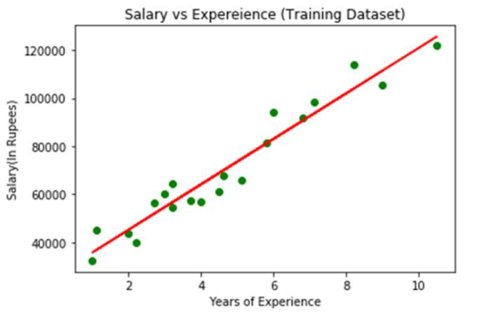
The real values observed are shown in green dots in the image above, while the anticipated values are enclosed by the red regression line. The relationship of the dependent and independent variables is depicted by the regression line.
Calculating the gap between the actual values and the anticipated values allows one to see how well the line fits the data. However, as we can see from the plot above, the majority of the observations are near to the regression line, hence our model works well for the training set.
Step 5. Showing The Outcomes Of The Test Set
We visualized our model's performance on the training set in the preceding phase. We will now repeat the process for the Test set. The entire program will be identical to the one above, with the exception that a test and b test will be used in place of a train and b train.
<div class="code-mirror  language-python" contenteditable="plaintext-only" spellcheck="false" style="outline: none; overflow-wrap: break-word; overflow-y: auto; white-space: pre-wrap;">mtplt<span class="token punctuation">.</span>scatter<span class="token punctuation">(</span>a_train<span class="token punctuation">,</span> b_train<span class="token punctuation">,</span> color<span class="token operator">=</span><span class="token string">"blue"</span><span class="token punctuation">)</span>
mtplt<span class="token punctuation">.</span>plot<span class="token punctuation">(</span>a_train<span class="token punctuation">,</span> a_pred<span class="token punctuation">,</span> color<span class="token operator">=</span><span class="token string">"red"</span><span class="token punctuation">)</span>
mtplt<span class="token punctuation">.</span>title<span class="token punctuation">(</span><span class="token string">"Salary vs Experience (Test Dataset)"</span><span class="token punctuation">)</span>
mtplt<span class="token punctuation">.</span>xlabel<span class="token punctuation">(</span><span class="token string">"Years of Experience"</span><span class="token punctuation">)</span>
mtplt<span class="token punctuation">.</span>ylabel<span class="token punctuation">(</span><span class="token string">"Salary(In Rupees)"</span><span class="token punctuation">)</span>
mtplt<span class="token punctuation">.</span>show<span class="token punctuation">(</span><span class="token punctuation">)</span>
</div>
Output
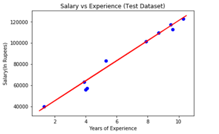
The blue color in the plot above represents observations, and the red regression line represents predictions. We can state that our Simple Linear Regression is a solid model and capable of making good predictions because, as we can see, the majority of the variables are close to the regression line.
Conclusion
Every machine learning enthusiast has to be familiar with the linear regression algorithm, and beginners to machine learning should start there. It's a fairly straightforward but helpful algorithm. We hope you found this information to be useful.

3K+ Views
