Scalable Data Processing in R

Most of the time, the R programmers encounter large data that causes problems as by default variables are stored in the memory. The R language doesn’t work well with a huge amount of data larger than 10% of the computer’s RAM. But data processing should be scalable if we want to excel in the field of data science. So, we will discuss how we can apply certain operations and use scalable data processing easily when the data is sufficiently larger than the computer’s RAM. The discussion would also be focussed on dealing with “out of core” objects.

What is Scalable data processing?

Scalability is a very important aspect when big data comes into the picture. As we know, it takes more time to read and write data into a disk than to read and write data into RAM. Because of this, it takes a lot of time when we need to retrieve some data from a hard disk as compared to RAM. The computer’s resources like RAM, processors, and hard drives play a major role in deciding how fast our R code executes. As we know that we cannot change such resources (except replacing them with new hardware) but we can make use of these resources in an efficient way.

For example, let us consider that we have a dataset that is equal to the size of the RAM. The cost could be cut by loading only the part of the dataset that we actually require at the moment.

Relationship between processing time and the data size

The processing time depends upon the size of the dataset. The larger dataset generally takes a longer time to process. But it is important to note that the processing time is not directly proportional to the size of the dataset.

Let us understand in simple words by taking an example. Suppose we have two datasets out of which one is twice the size of the other. So, the time taken to process the larger dataset is not twice the time taken to process the other dataset.

The processing time for the larger dataset would obviously be more than the smaller one but we cannot clearly say that it would be twice the smaller one or three times etc. It totally depends upon the operations being performed on the dataset elements.

R provides us a microbenchmark package that can be used to compare the timing of two or more operations. We can also plot the difference using plot() function in R.

Example

For example, consider the following program that sorts random arrays of different sizes −

# Load the microbenchmark package
library(microbenchmark)

# Time comparison between sorting vectors of 
# different sizes
microbenchmarkObject <- microbenchmark(
  
   # Sort a random normal vector length 5e5
   "5e5" = sort(rnorm(5e5)),
     
   # Sort a random normal vector length 4e5
   "4e5" = sort(rnorm(4e5)),
     
   # Sort a random normal vector length 3e5
   "3e5" = sort(rnorm(3e5)),
     
   # Sort a random normal vector length 2e5  
   "2e5" = sort(rnorm(2e5)),
     
   # Sort a random normal vector length 1e6  
   "1e6" = sort(rnorm(1e6)),
   times = 15
)

# Plot the resulting benchmark object
plot(microbenchmarkObject)

Output

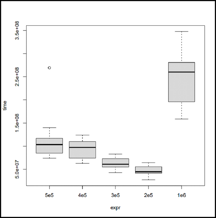
As you can see in the output, the execution time does not come out to be the same every time. The reason for this is that while the system is executing the R code, other things are also going under the hood.

Note that it is also a good practice to keep the track of the operations using the microbenchmark library while evaluating the execution time of R code.

Working with "out of core" Objects

In this section, we will discuss the big.matrix object. The big.matrix comprises an object in R that does more or less the same as the data structure in C++. This object seems like a generic R matrix but prevents developers from memory-consuming problems of a generic R matrix.

Now we will create our own big.matrix object using the read.big.matrix() function.

The function is also quite similar to read.table() but it requires us to specify the type of value we want to read i.e, “char”, “short”, “integer”, “double”. The name of the file must be given to hold the matrix’s data (the backing file), and it needs the name of the file to hold information about the matrix (a descriptor file). The outcome will be stored in a file on the disk that keeps the value read with a descriptor file that keeps more description about the resulting big.matrix object.

Installing bigmemory library

Before moving further, we need to install the “bigmemory” library. You can download this library using the following command in CRAN −

install.packages("bigmemory")

Importing bigmemory

The first step is to import the bigmemory library. Import the library using the following command −

library(bigmemory)

Downloading the File

Now download a sample csv file "mortgage-sample.csv" −

# Download file using URL
download.file("http://s3.amazonaws.com/assets.datacamp.com/production/course_2399/datasets/mortgage-sample.csv", destfile = "mortgage-sample.csv")

Creating big.matrix object

We will now create an object of big.matrix. For this purpose, the argument passed is going to be “mortgage-sample.desc”. The dimension of the object can be extracted using dim() function −

Example

# Create an object of 
object <- read.big.matrix("mortgage-sample.csv", header = TRUE, type = "integer",
   descriptorfile = "mortgage-sample.desc")

# Display the dimensions
dim(object)

Output

[1] 70000    16

As you can see in the output, sizes of the big.matrix object have been displayed.

Display big.matrix object

To display the first 6 rows, we can use the head() function −

Example

head(object)

Output

     enterprise record_number msa perc_minority
[1,]          1           566   1             1
[2,]          1           116   1             3
[3,]          1           239   1             2
[4,]          1            62   1             2
[5,]          1           106   1             2
[6,]          1           759   1             3
     tract_income_ratio borrower_income_ratio
[1,]                  3                     1
[2,]                  2                     1
[3,]                  2                     3
[4,]                  3                     3
[5,]                  3                     3
[6,]                  3                     2
     loan_purpose federal_guarantee borrower_race
[1,]            2                 4             3
[2,]            2                 4             5
[3,]            8                 4             5
[4,]            2                 4             5
[5,]            2                 4             9
[6,]            2                 4             9
     co_borrower_race borrower_gender
[1,]                9               2
[2,]                9               1
[3,]                5               1
[4,]                9               2
[5,]                9               3
[6,]                9               1
     co_borrower_gender num_units affordability year
[1,]                  4         1             3 2010
[2,]                  4         1             3 2008
[3,]                  2         1             4 2014
[4,]                  4         1             4 2009
[5,]                  4         1             4 2013
[6,]                  2         2             4 2010
     type
[1,]    1
[2,]    1
[3,]    0
[4,]    1
[5,]    1
[6,]    1

Creating Table

We can also create a table. The sample csv file contains year as the column name, so we can display the number of mortgages using the following program −

Example

# Create a table for the number
# of mortages for each specific year
print(table(object[, "year"]))

Output

2008 2009 2010 2011 2012 2013 2014 2015 
6919 8996 7269 6561 8932 8316 4687 5493 

As you can see in the output, the number of mortgages have been displayed for each specific year.

Data Summary

Now we have learnt how we can import a big.matrix object. We will now see how we can analyze the data stored in the object. R provides us binanalytics package using which we can create summaries. You can download biganalytics library using the following in CRAN −

install.packages("biganalytics")

Example

Now let us consider the following program that displays the summary of the mortgage −

library(biganalytics)

# Download file using URL
download.file("http://s3.amazonaws.com/assets.datacamp.com/production/course_2399/datasets/mortgage-sample.csv", 
   destfile = "mortgage-sample.csv")

# Create an object of 
object <- read.big.matrix("mortgage-sample.csv", 
   header = TRUE, 
   type = "integer",
   descriptorfile = "mortgage-sample.desc")

# Display the summary
summary(object)

Output

enterprise               1.0000000    2.0000000    1.3814571    0.0000000
record_number            0.0000000  999.0000000  499.9080571    0.0000000
msa                      0.0000000    1.0000000    0.8943571    0.0000000
perc_minority            1.0000000    9.0000000    1.9701857    0.0000000
tract_income_ratio       1.0000000    9.0000000    2.3431571    0.0000000
borrower_income_ratio    1.0000000    9.0000000    2.6898857    0.0000000
loan_purpose             1.0000000    9.0000000    3.7670143    0.0000000
federal_guarantee        1.0000000    4.0000000    3.9840857    0.0000000
borrower_race            1.0000000    9.0000000    5.3572429    0.0000000
co_borrower_race         1.0000000    9.0000000    7.0002714    0.0000000
borrower_gender          1.0000000    9.0000000    1.4590714    0.0000000
co_borrower_gender       1.0000000    9.0000000    3.0494857    0.0000000
num_units                1.0000000    4.0000000    1.0398143    0.0000000
affordability            0.0000000    9.0000000    4.2863429    0.0000000
year                  2008.0000000 2015.0000000 2011.2714714    0.0000000
type                     0.0000000    1.0000000    0.5300429    0.0000000

The output shows the summary of the object by specifying min, max, mean, and NAs values.

Conclusion

In this tutorial, we discussed scalable data processing in R. We started with how processing time is related to data size. We saw the working of “out of core” objects like big.matrix. I hope through this tutorial you would have gained the knowledge of scalable data processing in R which is important from the perspective of data science.