- ML - Home
- ML - Introduction
- ML - Getting Started
- ML - Basic Concepts
- ML - Ecosystem
- ML - Python Libraries
- ML - Applications
- ML - Life Cycle
- ML - Required Skills
- ML - Implementation
- ML - Challenges & Common Issues
- ML - Limitations
- ML - Reallife Examples
- ML - Data Structure
- ML - Mathematics
- ML - Artificial Intelligence
- ML - Neural Networks
- ML - Deep Learning
- ML - Getting Datasets
- ML - Categorical Data
- ML - Data Loading
- ML - Data Understanding
- ML - Data Preparation
- ML - Models
- ML - Supervised Learning
- ML - Unsupervised Learning
- ML - Semi-supervised Learning
- ML - Reinforcement Learning
- ML - Supervised vs. Unsupervised
Machine Learning Data Visualization
- ML - Data Visualization
- ML - Histograms
- ML - Density Plots
- ML - Box and Whisker Plots
- ML - Correlation Matrix Plots
- ML - Scatter Matrix Plots
Statistics for Machine Learning
- ML - Statistics
- ML - Mean, Median, Mode
- ML - Standard Deviation
- ML - Percentiles
- ML - Data Distribution
- ML - Skewness and Kurtosis
- ML - Bias and Variance
- ML - Hypothesis
Regression Analysis In ML
- ML - Regression Analysis
- ML - Linear Regression
- ML - Simple Linear Regression
- ML - Multiple Linear Regression
- ML - Polynomial Regression
- ML - Classification Algorithms
- ML - Logistic Regression
- ML - K-Nearest Neighbors (KNN)
- ML - Naïve Bayes Algorithm
- ML - Decision Tree Algorithm
- ML - Support Vector Machine
- ML - Random Forest
- ML - Confusion Matrix
- ML - Stochastic Gradient Descent
- ML - Clustering Algorithms
- ML - Centroid-Based Clustering
- ML - K-Means Clustering
- ML - K-Medoids Clustering
- ML - Mean-Shift Clustering
- ML - Hierarchical Clustering
- ML - Density-Based Clustering
- ML - DBSCAN Clustering
- ML - OPTICS Clustering
- ML - HDBSCAN Clustering
- ML - BIRCH Clustering
- ML - Affinity Propagation
- ML - Distribution-Based Clustering
- ML - Agglomerative Clustering
- ML - Dimensionality Reduction
- ML - Feature Selection
- ML - Feature Extraction
- ML - Backward Elimination
- ML - Forward Feature Construction
- ML - High Correlation Filter
- ML - Low Variance Filter
- ML - Missing Values Ratio
- ML - Principal Component Analysis
- ML - Reinforcement Learning Algorithms
- ML - Exploitation & Exploration
- ML - Q-Learning
- ML - REINFORCE Algorithm
- ML - SARSA Reinforcement Learning
- ML - Actor-critic Method
- ML - Monte Carlo Methods
- ML - Temporal Difference
- ML - Deep Reinforcement Learning
- ML - Deep Reinforcement Learning Algorithms
- ML - Deep Q-Networks
- ML - Deep Deterministic Policy Gradient
- ML - Trust Region Methods
- ML - Performance Metrics
- ML - Automatic Workflows
- ML - Boost Model Performance
- ML - Gradient Boosting
- ML - Bootstrap Aggregation (Bagging)
- ML - Cross Validation
- ML - AUC-ROC Curve
- ML - Grid Search
- ML - Data Scaling
- ML - Train and Test
- ML - Association Rules
- ML - Apriori Algorithm
- ML - Gaussian Discriminant Analysis
- ML - Cost Function
- ML - Bayes Theorem
- ML - Precision and Recall
- ML - Adversarial
- ML - Stacking
- ML - Epoch
- ML - Perceptron
- ML - Regularization
- ML - Overfitting
- ML - P-value
- ML - Entropy
- ML - MLOps
- ML - Data Leakage
- ML - Monetizing Machine Learning
- ML - Types of Data
Classification Algorithms In ML
Clustering Algorithms In ML
Dimensionality Reduction In ML
Reinforcement Learning
Deep Reinforcement Learning
Quantum Machine Learning
Machine Learning Miscellaneous
Machine Learning - Resources
Machine Learning - Simple Linear Regression
What is Simple Linear Regression?
Simple linear regression is a statistical and supervised learning method in which a single independent variable (also known as a predictor variable) is used to predict the dependent variable. In other words, it models the linear relationship between the dependent variable and a single independent variable.
Simple linear regression in machine learning is a type of linear regression. When the linear regression algorithm deals with a single independent variable, it is known as simple linear regression. When there is more than one independent variable (feature variables), it is known as multiple linear regression.
Independent Variable
The feature inputs in the dataset are termed as the independent variables. There is only a single independent variable in simple linear regression. An independent variable is also known as a predictor variable as it is used to predict the target value. It is plotted on a horizontal axis.
Dependent Variable
The target value in the dataset is termed as the dependent variable. It is also known as a response variable or predicted variable. It is plotted on a vertical axis.
Line of Regression
In simple linear regression, a line of regression is a straight line that best fits the data points and is used to show the relationship between a dependent variable and an independent variable.
Graphical Representation
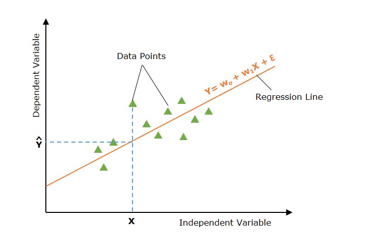
The following graph depicts the simple linear regression model −

In the above image, the straight line represents the simple linear regression line where Ŷ is the predicted value, and Y is dependent variable (target) and X is independent variable (input).
Simple Linear Regression Model
A simple linear regression model in machine learning can be represented as the following mathematical equation −
$$\mathrm{ Y = w_0 + w_1 X + \epsilon }$$
Where
- Y is the dependent variable (target).
- X is the independent variable (feature).
- w0 is the y-intercept of the line.
- w1 is the slope of the line, representing the effect of X on Y.
- õ is the error term, capturing the variability in Y not explained by X.
How Simple Linear Regression Works?
The main of simple linear regression is to find the best fit line (a straight line) through the data points that minimizes the difference between the actual values and predicted values.
Defining Hypothesis Function
In simple linear regression, the hypothesis is that there is a linear relation between the dependent variable (output/ target) and the independent variable (input). This linear relation can be represented using a linear equation −
$$\mathrm{\hat{Y} = w_0 + w_1 X}$$
With different values of parameters w0 and w1 there are multiple linear equations (straight lines). The set of all such linear equations (all straight lines) is termed hypothesis space.
Now, the main aim of the simple linear regression model is to find the best-fit line in Hypothesis space (set of all straight lines).
Finding the Best Fit Line
Now the task is to find the best fit line (line of regression). To do this, we define a cost function or loss function that measure the the difference between the actual values and predicted values.
To find the best fit line, the simple linear regression model initializes (with default values) the parameters of the regression line. This regression line (with initialized parameters) is used to find the predicted values for the given input values.
Loss Function for Simple Linear Regression
Now using the input and predicted values, we compute the loss function. The loss function is used to find the optimal values of the parameters.
The loss function finds the difference between the input value and predicted value. There are different loss functions such as mean squared error (MSE), mean absolute error (MEA), R-squared, etc. used in simple linear regression. The most commonly used loss function is mean squared error.
The loss function for simple linear regression in terms of mean squared error is as follows −
$$\mathrm{J(w_0, w_1) = \frac{1}{2n} \sum_{i=1}^{n} \left( Y_i - \hat{Y}_i \right)^2}$$
Optimization
The optimal values of parameters are those values that minimize the cost function. Finding the optimal values is an iterative process in which the parameters are updated iteratively.
There are many optimization techniques applied in simple linear regression. Gradient Descent is a simple and most common optimization technique used in simple linear regression.
A linear equation with optimal parameter values is the best fit line(regression line) and it is the final solution for a simple linear regression problem. This line is used to predict new and unseen data.
Assumptions of Simple Linear Regression
There are some assumptions about the dataset that are made by the simple linear regression model. The following are some assumptions −
- Linearity − This assumption assumes that the relationship between the dependent and independent variables is linear. That means the dependent variable changes linearly as the independent variable changes. A scatter plot will show the linearity in the dataset.
- Homoskedasticity − For all observations, the variance of the residuals is the same. This assumption relates to the squared residuals.
- Independence − The examples (observations or X and Y pairs) are independent. There is no collinearity in data so the residuals will not be correlated. To check this, we example the scatter plot of residuals vs. fits.
- Normality − Model Residuals are normally distributed. Residuals are the differences between the actual and predicted values. To check for the normality, we examine the histogram of residuals. The histogram should be approximately normally distributed.
Implementation of Simple Linear Regression Algorithm using Python
To implement the simple linear regression algorithm, we are taking a dataset with two variables: YearsExperience (independent variable) and Salary (dependent variable).
Here, we are using the following dataset. The dataset contains 30 examples of data points. You can create a CSV file and store these data points in it.
Salary_Data.csv
| Years of Experience | Salary |
|---|---|
| 1.1 | 39343 |
| 1.3 | 46205 |
| 1.5 | 37731 |
| 2 | 43525 |
| 2.2 | 39891 |
| 2.9 | 56642 |
| 3 | 60150 |
| 3.2 | 54445 |
| 3.2 | 64445 |
| 3.7 | 57189 |
| 3.9 | 63218 |
| 4 | 55794 |
| 4 | 56957 |
| 4.1 | 57081 |
| 4.5 | 61111 |
| 4.9 | 67938 |
| 5.1 | 66029 |
| 5.3 | 83088 |
| 5.9 | 81363 |
| 6 | 93940 |
| 6.8 | 91738 |
| 7.1 | 98273 |
| 7.9 | 101302 |
| 8.2 | 113812 |
| 8.7 | 109431 |
| 9 | 105582 |
| 9.5 | 116969 |
| 9.6 | 112635 |
| 10.3 | 122391 |
| 10.5 | 121872 |
What is the purpose of this implementation?
The purpose of building this simple linear regression model is to determine which line best represents the relationship between the two variables.
The following are the steps to implement the simple linear regression model in Python −
Step 1: Data Preparation
Data preparation or pre-processing is the initial step. We have our dataset as a CSV file named "Salary_Data.csv," as discussed above.
We need to import python libraries prior to importing the dataset and building the simple linear regression model.
import numpy as np
import matplotlib.pyplot as plt
import pandas as pd
Load the dataset
dataset = pd.read_csv('Salary_Data.csv')
The dependent variable (X) and independent variable (Y) must then be extracted from the provided dataset. Years of experience (YearsExperience) is the independent variable, and Salary is the dependent variable.
X = dataset.iloc[:, :-1].values
y = dataset.iloc[:, -1].values
Let's check the first five examples of the dataset.
import numpy as np
import matplotlib.pyplot as plt
import pandas as pd

dataset = pd.read_csv('Salary_Data.csv')

X = dataset.iloc[:, :-1].values
y = dataset.iloc[:, -1].values

print(dataset.head())
Output
0	1.1	39343.0
1	1.3	46205.0
2	1.5	37731.0
3	2.0	43525.0
4	2.2	39891.0
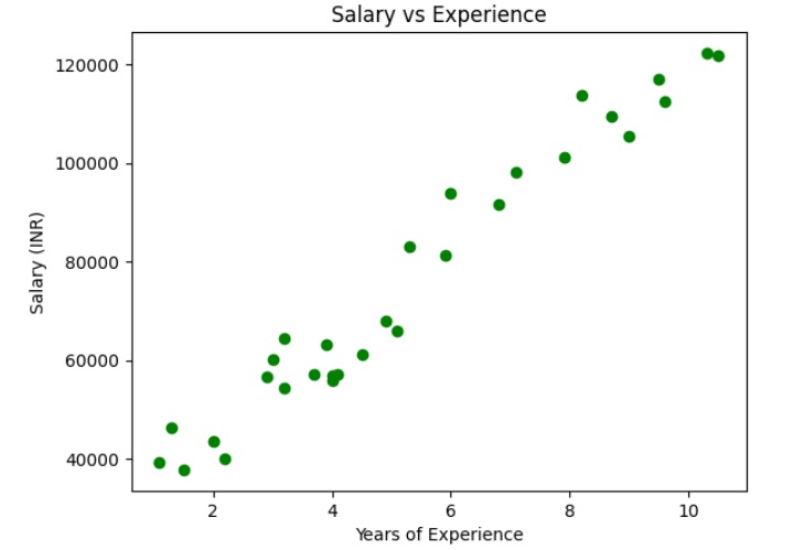
Lets check if the dataset is linear or not
import numpy as np
import matplotlib.pyplot as plt
import pandas as pd

dataset = pd.read_csv('Salary_Data.csv')

X = dataset.iloc[:, :-1].values
y = dataset.iloc[:, -1].values

plt.scatter(X, y, color="green")
plt.title("Salary vs Experience")
plt.xlabel("Years of Experience")
plt.ylabel("Salary (INR)")
plt.show()
Output

The above graph shows that the dependent and independent variables are linearly dependent. So we can apply the simple linear regression on the dataset to find the best relation between these variables.
Split the dataset into training and testing sets
The training set and test set will then be divided into two groups. We will use 80% observations for the training set and 20% observations for the test set out of the total 30 observations we have. So there will be 24 observation in training set and 6 observation in test set. We divide our dataset into training and test sets so that we can use one set to train and the other to test our model.
# Split the dataset into training and testing sets
from sklearn.model_selection import train_test_split
X_train, X_test, y_train, y_test = train_test_split(X, y, test_size = 0.2)
Here, X_train represents the input feature of the training data and y_train represents the output variable (target variable).
Step 2: Model Training (Fitting the Simple Linear Regression to Training Set)
The next step is fitting our model with the training dataset. We will use scikit-learn's LinearRegression class to train a simple linear regression model on the training data. The code for this is as follows −
from sklearn.linear_model import LinearRegression

# Create a linear regression object
regressor= LinearRegression()
regressor.fit(X_train, y_train)
The fit() method is used to fit the linear regression object (regressor) to the training data. The model learns the relation between the predictor variable (X_train), and the target variable (y_train).
Step 3: Model Testing
Once the model is trained, we can use it to make predictions on the test data. The code for this is as follows −
# Split the dataset into training and testing sets
from sklearn.model_selection import train_test_split
X_train, X_test, y_train, y_test = train_test_split(X, y, test_size = 0.2)

from sklearn.linear_model import LinearRegression

# Create a linear regression object
regressor= LinearRegression()
regressor.fit(X_train, y_train)

y_pred = regressor.predict(X_test)
df = pd.DataFrame({'Actual Values':y_test, 'Predicted Values':y_pred})
print(df)
Output
   Actual Values  Predicted Values
0              8          8.0
The above output shows actual values and predicted values of Salary in the test set.
Here, X_test represents the input feature of the test data and y_pred represents the predicted output variable (target variable).
Similarly, you can test the model with training data.
y_pred = regressor.predict(X_train)
df = pd.DataFrame({'Real Values':y_test, 'Predicted Values':y_pred})
print(df)
Output
    Real Values  Predicted Values
0       57189.0      60702.225094
1       64445.0      55981.813188
2       63218.0      62590.389857
3      122391.0     123011.662261
4       91738.0      89968.778915
5       43525.0      44652.824612
6       61111.0      68254.884145
7       56642.0      53149.566044
8       66029.0      73919.378433
9       83088.0      75807.543195
10      46205.0      38044.247943
11     109431.0     107906.344160
12      98273.0      92801.026059
13      37731.0      39932.412705
14      54445.0      55981.813188
15      39891.0      46540.989374
16     101302.0     100353.685109
17      55794.0      63534.472238
18      81363.0      81472.037483
19      39343.0      36156.083180
20     113812.0     103185.932253
21      67938.0      72031.213670
22     112635.0     116403.085592
23     105582.0     110738.591304
Step 4: Model Evaluation
We need to evaluate the performance of the model to determine its accuracy. We will use the mean squared error (MSE), root mse (RMSE), mean average error (MAE), and the coefficient of determination (R^2) as evaluation metrics. The code for this is as follows −
from sklearn.metrics import mean_squared_error
from sklearn.metrics import mean_absolute_error
from sklearn.metrics import r2_score

# get the predicted values for test dat
y_pred = regressor.predict(X_test)
mse = mean_squared_error(y_test, y_pred)
print("mse", mse)
rmse = mean_squared_error(y_test, y_pred)
print("rsme", rmse)
mae = mean_absolute_error(y_test, y_pred)
print("mae", mae)
Output
mse 7.888609052210118e-31
rsme 7.888609052210118e-31
mae 8.881784197001252e-16
Here, y_test represents the actual output variable of the test data.
Step 5: Visualize Training Set Results (with Regression Line)
Now, let's visualize the results on the training set and the regression line.
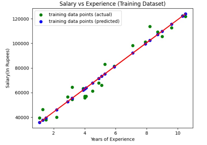
We use the scatter plot to plot the actual values (input and target values) in the training set. We also plot a straight line (regression line) for actual values (input) and predicted values of the training set.
# Split the dataset into training and testing sets
from sklearn.model_selection import train_test_split
X_train, X_test, y_train, y_test = train_test_split(X, y, test_size = 0.2)

from sklearn.linear_model import LinearRegression

y_pred = regressor.predict(X_train)
plt.scatter(X_train, y_train, color="green", label="training data points (actual)")
plt.scatter(X_train, y_pred, color="blue",label="training data points (predicted)")
plt.plot(X_train, y_pred, color="red")
plt.title("Salary vs Experience (Training Dataset)")
plt.xlabel("Years of Experience")
plt.ylabel("Salary(In Rupees)")
plt.legend()
plt.show()
Output

The above graph shows the line of regression (straight line in red color), actual values (in green color), and predicted values (in blue color) for the training set.
Step 6: Visualize the Test Set Results (with Regression Line)
Now, let's visualize the results on the test set and the regression line.
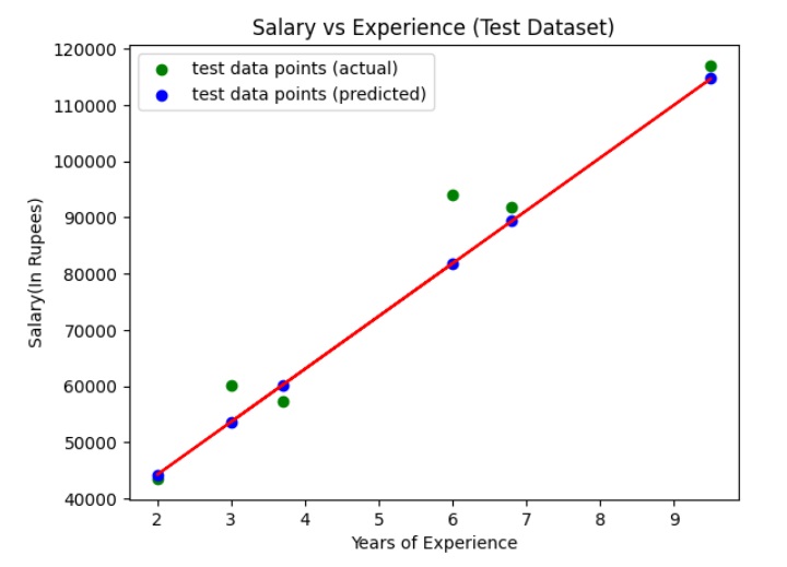
We use the scatter plot to plot the actual values (input and target values) in the test set. We also plot a straight line (regression line) for actual values (input) and predicted values of the test set.
# Split the dataset into training and testing sets
from sklearn.model_selection import train_test_split
X_train, X_test, y_train, y_test = train_test_split(X, y, test_size = 0.2)

from sklearn.linear_model import LinearRegression

y_pred = regressor.predict(X_test)
plt.scatter(X_test, y_test, color="green", label="test data points (actual)")
plt.scatter(X_test, y_pred, color="blue",label="test data points (predicted)")
plt.plot(X_test, y_pred, color="red")
plt.title("Salary vs Experience (Test Dataset)")
plt.xlabel("Years of Experience")
plt.ylabel("Salary(In Rupees)")
plt.legend()
plt.show()
Output

The above graph shows the line of regression (straight line in red color), actual values (in green color), and predicted values (in blue color) for the test set.