
Article Categories
- All Categories
-
 Data Structure
-
 Networking
-
 RDBMS
RDBMS
-
 Operating System
-
 Java
Java
-
 MS Excel
-
 iOS
iOS
-
 HTML
HTML
-
 CSS
CSS
-
 Android
-
 Python
-
 C Programming
-
 C++
C++
-
 C#
C#
-
 MongoDB
-
 MySQL
MySQL
-
 Javascript
-
 PHP
PHP
-
 Economics & Finance
Low Pass and High Pass Filter Bode Plot
The Bode Plot is the frequency response plot of linear systems represented in the form of logarithmic plots. In bode plot the horizontal axis represents frequency on a logarithmic scale and the vertical axis represents either the amplitude or the phase of the frequency response function.
Low Pass Filter Bode Plot
The frequency response function or transfer function of the RC low pass filter is given by,
$$\frac{V_{out}}{V_{in}}=\frac{A}{1+(j\omega\:T)}=\frac{A}{1+(j\omega\:/\omega_{0})}=\frac{A}{\sqrt{1+(\omega\:/\omega_{0})^{2}}}\angle\:-\tan^{-1}(\frac{\omega}{\omega_{0}})$$
Where,
T = Time constant of the circuit = $1/\omega_{0}=RC$
A = Constant and
$\omega_{0}$ = Cut off frequency
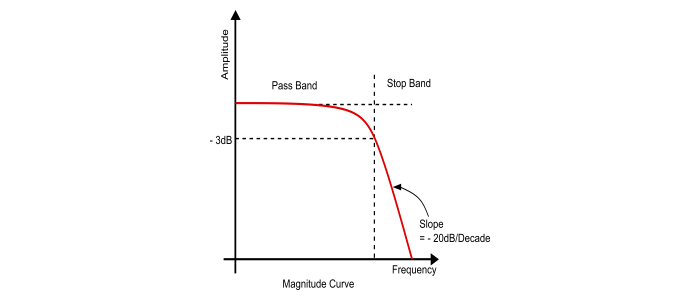
Bode Magnitude Plot of LPF
The magnitude plot can be obtained from the absolute value of transfer function i.e.
$$|\frac{V_{out}}{V_{in}}|=20\log_{10}\frac{|A|}{|1+j\omega\:/\omega_{0}|}$$
When $\omega\:
$$|\frac{V_{out}}{V_{in}}|_{dB}=20\log_{10}A-20\log_{10}\:1=20\log_{10}A$$
Hence, at very low frequencies the frequency response function is approximated by a straight line of zero slope, which is the low frequency asymptote of the Bode plot.
When $\omega\:>\omega_{0}$ then the imaginary part is much larger than its real part, so $|1+j\omega\:/\omega_{0}|=|j\omega\:/\omega_{0}|$, thus,
$$|\frac{V_{out}}{V_{in}}|_{dB}=20\log_{10}A-20\log_{10}\:(\omega\:/\omega_{0})=20\log_{10}A-20\log_{10}\omega-20\log_{10}\omega_{0}$$
Hence, at very high frequencies the frequency response function is approximated by a straight line of (- 20 dB / Decade) slope that intercepts the $\log\omega$ at $\log\:\omega_{0}$. This line is the high frequency asymptote of the bode plot.
When $\omega=\omega_{0}$,the real and imaginary part of the simple pole are equal, so $|1+j\omega\:+\omega_{0}|=|1+j|=\sqrt{2}$, thus,
$$|\frac{V_{out}}{V_{in}}|_{dB}=20\log_{10}A-20\log_{10}\sqrt{2}=20\log_{10}A-3dB$$
Hence, the magnitude plot is approximated by two straight lines intersecting at $\omega_{0}$.
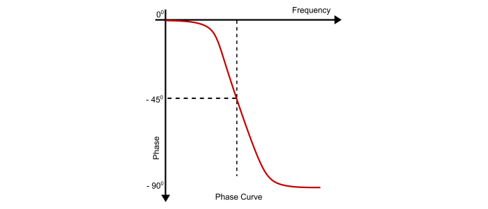
Bode Phase Plot of LPF
$$\angle(\frac{V_{out}}{V_{in}})=-\tan^{-1}(\frac{\omega}{\omega_{0}})$$
When $\omega\rightarrow0$, Then
$$\angle(\frac{V_{out}}{V_{in}})=-\tan^{-1}(\frac{\omega}{\omega_{0}})=0$$
When $\omega=0$, Then
$$\angle(\frac{V_{out}}{V_{in}})=-\tan^{-1}(\frac{\omega}{\omega_{0}})=-\frac{\pi}{4}$$
When $\omega\rightarrow\infty$, Then
$$\angle(\frac{V_{out}}{V_{in}})=-\tan^{-1}(\frac{\omega}{\omega_{0}})=-\frac{\pi}{2}$$
High Pass Filter Bode Plot
The frequency response or bode plot of the high pass filter is just opposite to that of bode plot of the low pass filter.
Using the transfer function or frequency response function of the filter circuit, we can plot the frequency response.
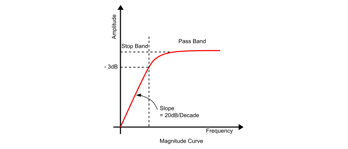
Bode Magnitude Plot of HPF
$$\frac{V_{out}}{V_{in}}(j\omega)|=\frac{\omega}{\sqrt{\omega^{2}+(\omega_{0})^{2}}}=\frac{\omega}{\sqrt{\omega^{2}+(1/RC)^{2}}}$$
When $\omega
When $\omega>\omega_{0}$, the filter circuit will allow the signal to pass and the region above the cut off frequency point is known as a pass band.
When $\omega=\omega_{0}$, at this point the amplitude of output voltage is 70.7% of the input voltage.
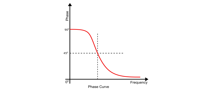
Bode Phase Plot of HPF
The phase plot can be obtained by the phase equation of the transfer function.
$$\angle(\frac{V_{out}}{V_{in}})=90^{\circ}-\tan^{-1}(\frac{\omega}{\omega_{0}})=90^{\circ}-\tan^{-1}(\omega\:RC)$$
When $\omega\rightarrow0$, Then
$$\angle(\frac{V_{out}}{V_{in}})=90^{\circ}-\tan^{-1}(\frac{\omega}{\omega_{0}})=\frac{\Pi}{2}$$
When $\omega=0$, Then
$$\angle(\frac{V_{out}}{V_{in}})=90^{\circ}-\tan^{-1}(\frac{\omega}{\omega_{0}})=\frac{\Pi}{4}$$
When $\omega\rightarrow\infty$, Then
$$\angle(\frac{V_{out}}{V_{in}})=90^{\circ}-\tan^{-1}(\frac{\omega}{\omega_{0}})=0$$

20K+ Views
