How to insert random(integer) numbers between two numbers without repeats in Excel?

In Microsoft Excel, when a user needs to produce random data or simulate scenarios, adding random integer numbers between two supplied numbers without repeats can be useful. Using this method, a user can fill a range with distinct random integers that fall inside a given range. This article will offer a step-by-step explanation, guaranteeing precision at each junction. The directions have been made to be simple to understand. Look at how to input random integer numbers in Excel without having them repeat.

Example 1: To Insert Specific Number of Rows at Fixed Intervals in Excel

Step 1

In Microsoft Excel, either create a new worksheet or open an existing one that contains the user's desired changes to the data.

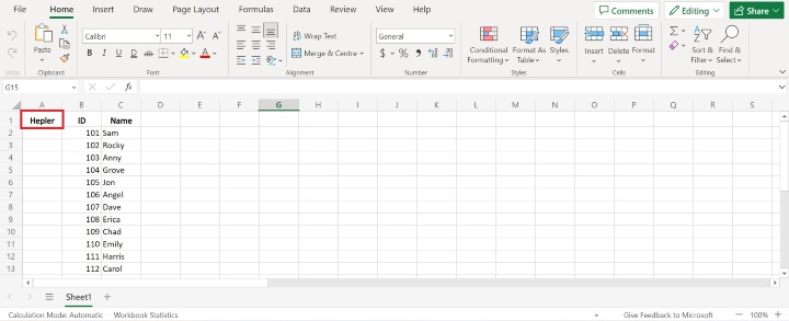
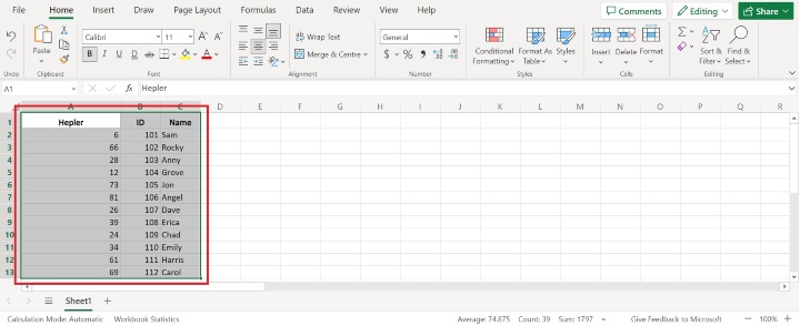
Open Microsoft Excel before beginning to create a new worksheet. Look for the tabs at the bottom of the Excel window. By default, a sheet named "Sheet1" is visible. Consider the illustration below for correct reference −

Add user data to the worksheet's cells. The data can be manually typed into the cells or copied and pasted from a different place. Consider the illustration below for correct reference −

Step 2

Select the range of numbers from which the user wants to produce random integers. Let’s take the scenario where the user wants to insert 100 random integers as an example. Also, decide how many random integers the user wants to produce in total; in this case, here assume 50.

Make a helper column and place it next to the data in an empty column. Random numbers will be produced using this column. Consider the illustration below for correct reference −

Step 3

Enter the formula =RANDBETWEEN(starting_number, ending_number) in the first cell of the helper column. Simply swap out "starting_number" for the lower value in the range and "ending_number" for the higher value. The equation can look like this =RANDBETWEEN(1, 100).

Consider the illustration below for correct reference −

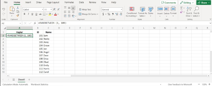
To generate a random integer between two given numbers, use the RANDBETWEEN formula in Microsoft Excel. When users need to create test data, simulate scenarios, or conduct random sampling in their spreadsheets, it is especially helpful. The starting number and the ending number, which specify the range within which the random number will be created, are the two inputs required by the formula.

Step 4

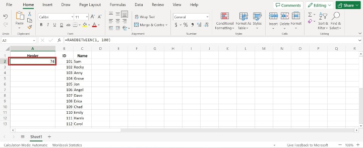
After writing the formula press enter. The random value will appear. Consider the illustration below for correct reference −

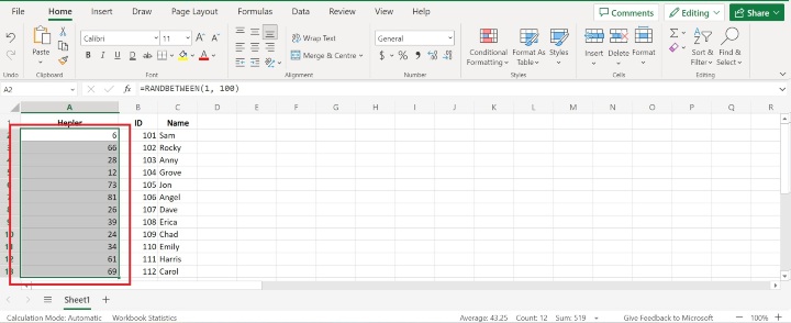
To apply the formula to all the cells in the helper column, pick the first cell of the column's formula and drag the fill handle down. Each cell will receive a random decimal number within the specified range as a result. Consider the illustration below for correct reference −

Step 5

Choose every row of information, including the support column. For appropriate reference, take into account the image below −

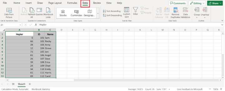
Now go to the "Data" tab. For accurate reference, look at the image below −

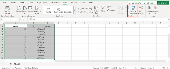
Now click on the "Remove Duplicates" button and print in "Data Tools". For appropriate reference, take into account the image below −

Right-click to select the full helpful column selection and then select "Copy." After that, paste the values where the user wants the random numbers to appear. The formulas are transformed into static values in this stage, ensuring that the numbers stay constant and do not change with each new computation.

Conclusion

In Excel, the user has successfully inserted random integer numbers without repeats between two given values. The user can create a distinct collection of random integers inside a specified range by following the detailed procedure described above. This method is useful in a variety of situations, such as data simulation, analysis, or the creation of test data.