
Article Categories
- All Categories
-
 Data Structure
-
 Networking
-
 RDBMS
RDBMS
-
 Operating System
-
 Java
Java
-
 MS Excel
-
 iOS
iOS
-
 HTML
HTML
-
 CSS
CSS
-
 Android
-
 Python
-
 C Programming
-
 C++
C++
-
 C#
C#
-
 MongoDB
-
 MySQL
MySQL
-
 Javascript
-
 PHP
PHP
-
 Economics & Finance
How to calculate the average in a column based on criteria in another column in Excel?
It is quite easy to find the average in a column based on the criteria in another column in an Excel sheet. In this tutorial, we will show how you can do it in just two simple steps.
Step 1
Open a Microsoft excel sheet, and enter the data as per your wish below I have considered this data as shown in the below screenshot for your reference. Here the excel contains the date, region and the values for the sales.

Step 2
Now you need to select a blank cell in an excel sheet and enter the below given formula and then press enter key or press the ctrl + shift+ enter key all at once as shown in the below screenshot for your reference.
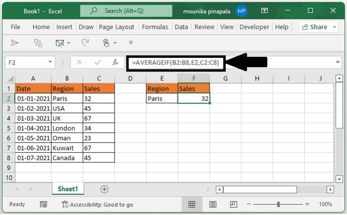
Note ? In the above-given formula, B2:B8 is the range that has the criteria and C2:C8 is the range that has the data that you want to calculate the average, for Paris you have calculated the average based on given information. You can change them as per your need.
Now the sales average of Paris is calculated. If you want to calculate the average of other values in the B column, then you have to repeat the above operation till all values averages are calculated.
Conclusion
In this tutorial, we used a simple example to demonstrate how you can use a formula to calculate the average in a column based on the criteria in another column in a Microsoft Excel sheet.

448 Views
