
Article Categories
- All Categories
-
 Data Structure
-
 Networking
-
 RDBMS
RDBMS
-
 Operating System
-
 Java
Java
-
 MS Excel
-
 iOS
iOS
-
 HTML
HTML
-
 CSS
CSS
-
 Android
-
 Python
-
 C Programming
-
 C++
C++
-
 C#
C#
-
 MongoDB
-
 MySQL
MySQL
-
 Javascript
-
 PHP
PHP
-
 Economics & Finance
How can Logistic Regression be implemented using TensorFlow?
Tensorflow is a machine learning framework that is provided by Google. It is an open-source framework used in conjunction with Python to implement algorithms, deep learning applications and much more. It is used in research and for production purposes. It has optimization techniques that help in performing complicated mathematical operations quickly. This is because it uses NumPy and multi-dimensional arrays.
Multi−dimensional arrays are also known as ‘tensors’. The framework supports working with deep neural network. It is highly scalable, and comes with many popular datasets. It uses GPU computation and automates the management of resources.
The ‘tensorflow’ package can be installed on Windows using the below line of code −
pip install tensorflow
Tensor is a data structure used in TensorFlow. It helps connect edges in a flow diagram. This flow diagram is known as the ‘Data flow graph’. Tensors are nothing but multidimensional array or a list.
The MNIST dataset contains handwritten digits, wherein 60000 of them are used for training the model and 10000 of them are used to test the trained model. These digits have been size−normalized and centered to fit a fixed-size image.
Following is an example −
Example
from __future__ import absolute_import, division, print_function
import tensorflow as tf
import numpy as np
num_classes = 10
num_features = 784
learning_rate = 0.01
training_steps = 1000
batch_size = 256
display_step = 50
from tensorflow.keras.datasets import mnist
(x_train, y_train), (x_test, y_test) = mnist.load_data()
x_train, x_test = np.array(x_train, np.float32), np.array(x_test, np.float32)
x_train, x_test = x_train.reshape([-1, num_features]), x_test.reshape([−1, num_features])
x_train, x_test = x_train / 255., x_test / 255.
train_data = tf.data.Dataset.from_tensor_slices((x_train, y_train))
train_data = train_data.repeat().shuffle(5000).batch(batch_size).prefetch(1)
A = tf.Variable(tf.ones([num_features, num_classes]), name="weight")
b = tf.Variable(tf.zeros([num_classes]), name="bias")
def logistic_reg(x):
return tf.nn.softmax(tf.matmul(x, A) + b)
def cross_entropy(y_pred, y_true):
y_true = tf.one_hot(y_true, depth=num_classes)
y_pred = tf.clip_by_value(y_pred, 1e−9, 1.)
return tf.reduce_mean(−tf.reduce_sum(y_true * tf.math.log(y_pred),1))
def accuracy_val(y_pred, y_true):
correct_prediction = tf.equal(tf.argmax(y_pred, 1), tf.cast(y_true, tf.int64))
return tf.reduce_mean(tf.cast(correct_prediction, tf.float32))
optimizer = tf.optimizers.SGD(learning_rate)
def run_optimization(x, y):
with tf.GradientTape() as g:
pred = logistic_reg(x)
loss = cross_entropy(pred, y)
gradients = g.gradient(loss, [A, b])
optimizer.apply_gradients(zip(gradients, [A, b]))
for step, (batch_x, batch_y) in enumerate(train_data.take(training_steps), 1):
run_optimization(batch_x, batch_y)
if step % display_step == 0:
pred = logistic_regression(batch_x)
loss = cross_entropy(pred, batch_y)
acc = accuracy_val(pred, batch_y)
print("step: %i, loss: %f, accuracy: %f" % (step, loss, acc))
pred = logistic_reg(x_test)
print("Test accuracy is : %f" % accuracy_val(pred, y_test))
import matplotlib.pyplot as plt
n_images = 4
test_images = x_test[:n_images]
predictions = logistic_reg(test_images)
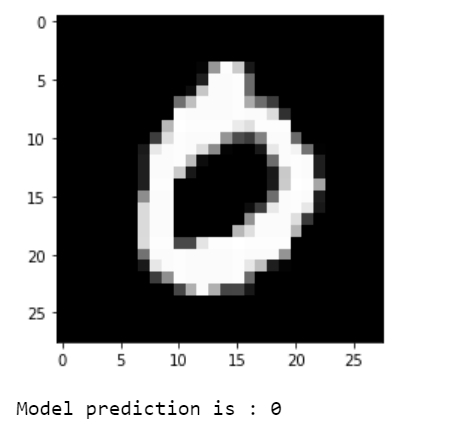
for i in range(n_images):
plt.imshow(np.reshape(test_images[i], [28, 28]), cmap='gray')
plt.show()
print("Model prediction is : %i" % np.argmax(predictions.numpy()[i]))
Code credit &minus https://github.com/aymericdamien/TensorFlow-Examples/blob/master/tensorflow_v2/notebooks/2_BasicModels/logistic_regression.ipynb
Output
step: 50, loss: 2.301992, accuracy: 0.132812
step: 100, loss: 2.301754, accuracy: 0.125000
step: 150, loss: 2.303200, accuracy: 0.117188
step: 200, loss: 2.302409, accuracy: 0.117188
step: 250, loss: 2.303324, accuracy: 0.101562
step: 300, loss: 2.301391, accuracy: 0.113281
step: 350, loss: 2.299984, accuracy: 0.140625
step: 400, loss: 2.303896, accuracy: 0.093750
step: 450, loss: 2.303662, accuracy: 0.093750
step: 500, loss: 2.297976, accuracy: 0.148438
step: 550, loss: 2.300465, accuracy: 0.121094
step: 600, loss: 2.299437, accuracy: 0.140625
step: 650, loss: 2.299458, accuracy: 0.128906
step: 700, loss: 2.302172, accuracy: 0.117188
step: 750, loss: 2.306451, accuracy: 0.101562
step: 800, loss: 2.303451, accuracy: 0.109375
step: 850, loss: 2.303128, accuracy: 0.132812
step: 900, loss: 2.307874, accuracy: 0.089844
step: 950, loss: 2.309694, accuracy: 0.082031
step: 1000, loss: 2.302263, accuracy: 0.097656
Test accuracy is : 0.869700
Explanation
The required packages are imported and aliased.
The learning parameters of the MNIST dataset are defined.
The MNIST dataset is loaded from the source.
The dataset is split into training and testing dataset. The images in the dataset are flattened to be shown as a 1−d vector that has 28 x 28 = 784 features.
The image values are normalized to contain [0,1] instead of [0,255].
A function named ‘logistic_reg’ is defined that gives the softmax value of the input data. It normalizes the logits to contain a probability distribution.
The cross entropy loss function is defined, that encodes the label to a one hot vector. The prediction values are formatted to reduce the log(0) error.
The accuracy metric needs to be computed, hence a function is defined.
The stochastic gradient descent optimizer is defined.
A function for optimization is defined, that computes gradients and updates the value of weights and bias.
The data is trained for a specified number of steps.
The built model is tested on the validation set.
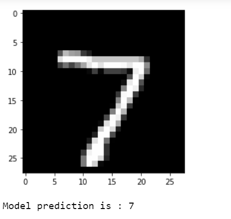
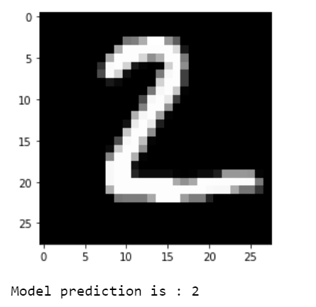
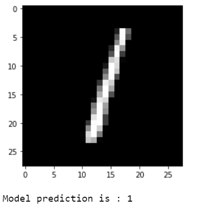
The predictions are visualized.

425 Views
