- Electrical Machines - Home
- Basic Concepts
- Electromechanical Energy Conversion
- Energy Stored in Magnetic Field
- Singly-Excited and Doubly Excited Systems
- Rotating Electrical Machines
- Electrical Machines Types
- Faraday’s Laws of Electromagnetic Induction
- Concept of Induced EMF
- Fleming's Left Hand and Right Hand Rules
- Transformers
- Electrical Transformer
- Construction of Transformer
- EMF Equation of Transformer
- Turns Ratio and Voltage Transformation Ratio
- Ideal Transformer
- Practical Transformer
- Ideal and Practical Transformers
- Transformer on DC
- Losses in a Transformer
- Efficiency of Transformer
- 3-Phase Transformer
- Types of Transformers
- More on Transformers
- Transformer Working Principle
- Single-Phase Transformer Working Principle
- 3-Phase Transformer Principle
- 3-Phase Induction Motor Torque-Slip
- 3-Phase Induction Motor Torque-Speed
- 3-Phase Transformer Harmonics
- Double-Star Connection (3-6 Phase)
- Double-delta Connection (3-6 Phase)
- Transformer Ratios
- Voltage Regulation
- Delta-Star Connection (3-Phase)
- Star-Delta Connection (3-Phase)
- Autotransformer Conversion
- Back-to-back Test (Sumpner's Test)
- Transformer Voltage Drop
- Autotransformer Output
- Open and Short Circuit Test
- 3-Phase Autotransformer
- Star-Star Connection
- 6-Phase Diametrical Connections
- Circuit Test (Three-Winding)
- Potential Transformer
- Transformers Parallel Operation
- Open Delta (V-V) Connection
- Autotransformer
- Current Transformer
- No-Load Current Wave
- Transformer Inrush Current
- Transformer Vector Groups
- 3 to 12-Phase Transformers
- Scott-T Transformer Connection
- Transformer kVA Rating
- Three-Winding Transformer
- Delta-Delta Connection Transformer
- Transformer DC Supply Issue
- Equivalent Circuit Transformer
- Simplified Equivalent Circuit of Transformer
- Transformer No-Load Condition
- Transformer Load Condition
- OTI WTI Transformer
- CVT Transformer
- Isolation vs Regular Transformer
- Dry vs Oil-Filled
- DC Machines
- Construction of DC Machines
- Types of DC Machines
- Working Principle of DC Generator
- EMF Equation of DC Generator
- Derivation of EMF Equation DC Generator
- Types of DC Generators
- Working Principle of DC Motor
- Back EMF in DC Motor
- Types of DC Motors
- Losses in DC Machines
- Applications of DC Machines
- More on DC Machines
- DC Generator
- DC Generator Armature Reaction
- DC Generator Commutator Action
- Stepper vs DC Motors
- DC Shunt Generators Critical Resistance
- DC Machines Commutation
- DC Motor Characteristics
- Synchronous Generator Working Principle
- DC Generator Characteristics
- DC Generator Demagnetizing & Cross-Magnetizing
- DC Motor Voltage & Power Equations
- DC Generator Efficiency
- Electric Breaking of DC Motors
- DC Motor Efficiency
- Four Quadrant Operation of DC Motors
- Open Circuit Characteristics of DC Generators
- Voltage Build-Up in Self-Excited DC Generators
- Types of Armature Winding in DC Machines
- Torque in DC Motors
- Swinburne’s Test of DC Machine
- Speed Control of DC Shunt Motor
- Speed Control of DC Series Motor
- DC Motor of Speed Regulation
- Hopkinson's Test
- Permanent Magnet DC Motor
- Permanent Magnet Stepper Motor
- DC Servo Motor Theory
- DC Series vs Shunt Motor
- BLDC Motor vs PMSM Motor
- Induction Motors
- Introduction to Induction Motor
- Single-Phase Induction Motor
- 3-Phase Induction Motor
- Construction of 3-Phase Induction Motor
- 3-Phase Induction Motor on Load
- Characteristics of 3-Phase Induction Motor
- Speed Regulation and Speed Control
- Methods of Starting 3-Phase Induction Motors
- More on Induction Motors
- 3-Phase Induction Motor Working Principle
- 3-Phase Induction Motor Rotor Parameters
- Double Cage Induction Motor Equivalent Circuit
- Induction Motor Equivalent Circuit Models
- Slip Ring vs Squirrel Cage Induction Motors
- Single-Cage vs Double-Cage Induction Motor
- Induction Motor Equivalent Circuits
- Induction Motor Crawling & Cogging
- Induction Motor Blocked Rotor Test
- Induction Motor Circle Diagram
- 3-Phase Induction Motors Applications
- 3-Phase Induction Motors Torque Ratios
- Induction Motors Power Flow Diagram & Losses
- Determining Induction Motor Efficiency
- Induction Motor Speed Control by Pole-Amplitude Modulation
- Induction Motor Inverted or Rotor Fed
- High Torque Cage Motors
- Double-Cage Induction Motor Torque-Slip Characteristics
- 3-Phase Induction Motors Starting Torque
- 3-phase Induction Motor - Rotor Resistance Starter
- 3-phase Induction Motor Running Torque
- 3-Phase Induction Motor - Rotating Magnetic Field
- Isolated Induction Generator
- Capacitor-Start Induction Motor
- Capacitor-Start Capacitor-Run Induction Motor
- Winding EMFs in 3-Phase Induction Motors
- Split-Phase Induction Motor
- Shaded Pole Induction Motor
- Repulsion-Start Induction-Run Motor
- Repulsion Induction Motor
- PSC Induction Motor
- Single-Phase Induction Motor Performance Analysis
- Linear Induction Motor
- Single-Phase Induction Motor Testing
- 3-Phase Induction Motor Fault Types
- Synchronous Machines
- Introduction to 3-Phase Synchronous Machines
- Construction of Synchronous Machine
- Working of 3-Phase Alternator
- Armature Reaction in Synchronous Machines
- Output Power of 3-Phase Alternator
- Losses and Efficiency of an Alternator
- Losses and Efficiency of 3-Phase Alternator
- Working of 3-Phase Synchronous Motor
- Equivalent Circuit and Power Factor of Synchronous Motor
- Power Developed by Synchronous Motor
- More on Synchronous Machines
- AC Motor Types
- Induction Generator (Asynchronous Generator)
- Synchronous Speed Slip of 3-Phase Induction Motor
- Armature Reaction in Alternator at Leading Power Factor
- Armature Reaction in Alternator at Lagging Power Factor
- Stationary Armature vs Rotating Field Alternator Advantages
- Synchronous Impedance Method for Voltage Regulation
- Saturated & Unsaturated Synchronous Reactance
- Synchronous Reactance & Impedance
- Significance of Short Circuit Ratio in Alternator
- Hunting Effect Alternator
- Hydrogen Cooling in Synchronous Generators
- Excitation System of Synchronous Machine
- Equivalent Circuit Phasor Diagram of Synchronous Generator
- EMF Equation of Synchronous Generator
- Cooling Methods for Synchronous Generators
- Assumptions in Synchronous Impedance Method
- Armature Reaction at Unity Power Factor
- Voltage Regulation of Alternator
- Synchronous Generator with Infinite Bus Operation
- Zero Power Factor of Synchronous Generator
- Short Circuit Ratio Calculation of Synchronous Machines
- Speed-Frequency Relationship in Alternator
- Pitch Factor in Alternator
- Max Reactive Power in Synchronous Generators
- Power Flow Equations for Synchronous Generator
- Potier Triangle for Voltage Regulation in Alternators
- Parallel Operation of Alternators
- Load Sharing in Parallel Alternators
- Slip Test on Synchronous Machine
- Constant Flux Linkage Theorem
- Blondel's Two Reaction Theory
- Synchronous Machine Oscillations
- Ampere Turn Method for Voltage Regulation
- Salient Pole Synchronous Machine Theory
- Synchronization by Synchroscope
- Synchronization by Synchronizing Lamp Method
- Sudden Short Circuit in 3-Phase Alternator
- Short Circuit Transient in Synchronous Machines
- Power-Angle of Salient Pole Machines
- Prime-Mover Governor Characteristics
- Power Input of Synchronous Generator
- Power Output of Synchronous Generator
- Power Developed by Salient Pole Motor
- Phasor Diagrams of Cylindrical Rotor Moto
- Synchronous Motor Excitation Voltage Determination
- Hunting Synchronous Motor
- Self-Starting Synchronous Motor
- Unidirectional Torque Production in Synchronous Motor
- Effect of Load Change on Synchronous Motor
- Field Excitation Effect on Synchronous Motor
- Output Power of Synchronous Motor
- Input Power of Synchronous Motor
- V Curves & Inverted V Curves of Synchronous Motor
- Torque in Synchronous Motor
- Construction of 3-Phase Synchronous Motor
- Synchronous Motor
- Synchronous Condenser
- Power Flow in Synchronous Motor
- Types of Faults in Alternator
- Miscellaneous Topics
- Electrical Generator
- Determining Electric Motor Load
- Solid State Motor Starters
- Characteristics of Single-Phase Motor
- Types of AC Generators
- Three-Point Starter
- Four-Point Starter
- Ward Leonard Speed Control Method
- Pole Changing Method
- Stator Voltage Control Method
- DOL Starter
- Star-Delta Starter
- Hysteresis Motor
- 2-Phase & 3-Phase AC Servo Motors
- Repulsion Motor
- Reluctance Motor
- Stepper Motor
- PCB Motor
- Single-Stack Variable Reluctance Stepper Motor
- Schrage Motor
- Hybrid Schrage Motor
- Multi-Stack Variable Reluctance Stepper Motor
- Universal Motor
- Step Angle in Stepper Motor
- Stepper Motor Torque-Pulse Rate Characteristics
- Distribution Factor
- Electrical Machines Basic Terms
- Synchronizing Torque Coefficient
- Synchronizing Power Coefficient
- Metadyne
- Motor Soft Starter
- CVT vs PT
- Metering CT vs Protection CT
- Stator and Rotor in Electrical Machines
- Electric Motor Winding
- Electric Motor
- Useful Resources
- Quick Guide
- Resources
- Discussion
Electrical Machines - Quick Guide
Electromechanical Energy Conversion
Today, electrical energy is the most widely used form of energy for performing several industrial, commercial and domestic functions such as pumping water, fans, coolers, air conditioning, refrigeration, etc. Since, most of processes require the conversion of electrical energy into mechanical energy. Also, the mechanical energy is converted into electrical energy. Hence, this clears that we need a mechanism to convert the electrical energy into mechanical energy and mechanical energy into electrical energy and such a mechanism is known as electromechanical energy conversion device.
Electromechanical Energy Conversion Device
Thus, a device which can convert electrical energy into mechanical energy or mechanical energy into electrical energy is known as electromechanical energy conversion device. The electric generators and electric motors are the examples of electromechanical energy conversion device.
In any electromechanical energy conversion device, the conversion of electrical energy into mechanical energy and vice-versa takes place through the medium of an electric field or a magnetic field. Though, in most of the practical electromechanical energy conversion devices, magnetic field is used as the coupling medium between electrical and mechanical systems.
The electromechanical energy conversion devices can be classified into two types −
Gross motion devices (like motors and generators)
Incremental motion devices (such as electromagnetic relays, measuring instruments, loudspeakers, etc.)
The device which converts electrical energy into mechanical energy is known as electric motor. The device which converts mechanical energy into electrical energy is known as electric generator.
In an electric motor, when a current carrying conductor is placed in a changing (or rotating) magnetic field, the conductor experiences a mechanical force. In case of a generator, when a conductor moves in a magnetic field, an EMF is induced in the conductor. Although, these two electromagnetic effects occur simultaneously, when the energy conversion takes place from electrical to mechanical and vice-versa in all the electromechanical energy conversion devices.
Energy Balance Equation
The energy balance equation is an expression which shows the complete process of energy conversion. In an electromechanical energy conversion device, the total input energy is equal to the sum of three components −
Energy dissipated or lost
Energy stored
Useful output energy
Therefore, for an electric motor, the energy balance equation can be written as,
Electrical energy input = Energy dissipated + Energy stored + Mechanical energy output
Where,
The electrical energy input is the electricity supplied from the main supply.
Energy stored is equal to sum of the energy stored in the magnetic field and in the mechanical system in the form of potential and kinetic energies.
The energy dissipated is equal to sum of energy loss in electric resistance, energy loss in magnetic core (hysteresis loss + eddy current loss) and mechanical losses (windage and friction losses).
For an electric generator, the energy balance equation can be written as,
Mechanical energy input = Electrical energy output + Energy stored + Energy dissipated
Where, the mechanical energy input is the mechanical energy obtained from a turbine, engine, etc. to turn the shaft of the generator.
Energy Stored in a Magnetic Field
In the previous chapter, we discussed that in an electromechanical energy conversion device, there is a medium of coupling between electrical and mechanical systems. In most of practical devices, magnetic field is used as the coupling medium. Therefore, an electromechanical energy conversion device comprises an electromagnetic system. Consequently, the energy stored in the coupling medium is in the form of the magnetic field. We can calculate the energy stored in the magnetic field of an electromechanical energy conversion system as described below.
Consider a coil having N turns of conductor wire wound around a magnetic core as shown in Figure-1. This coil is energized from a voltage source of v volts.

By applying KVL, the applied voltage to the coil to given by,
$$\mathrm{\mathit{V\:=\:e\:+\:iR}\cdot \cdot \cdot (1)}$$
Where,
e is induced EMF in the coil due to electromagnetic induction.
R is the resistance of the coil circuit.
$\mathit{i}$ is the current flowing the coil.
The instantaneous power input to the electromagnetic system is given by,
$$\mathrm{\mathit{p}\:=\:\mathit{Vi\:=\:i\left ( e+iR \right )}}$$
$$\mathrm{\Rightarrow \mathit{p}\:=\:\mathit{ie+ i^{\mathrm{2}}}\mathit{R}\cdot \cdot \cdot (2)}$$
Now, let a direct voltage is applied to the circuit at time t = 0 and that at end of t = t1 seconds, and the current in the circuit has attained a value of I amperes. Then, during this time interval, the energy input the system is given by,
$$\mathrm{\mathit{W}_{in}\:=\:\int_{0}^{t_{\mathrm{1}}}\:\mathit{p\:dt}}$$
$$\mathrm{\Rightarrow \mathit{W}_{in}\:=\:\int_{0}^{t_{\mathrm{1}}}\:\mathit{ie\:dt}\:+\:\int_{0}^{t_{\mathrm{1}}}\mathit{i^{\mathrm{2}}R\:dt}\cdot \cdot \cdot (3)}$$
From Equation-3, it is clear that the total input energy consists of two parts −
The first part is the energy stored in the magnetic field.
The second part is the energy dissipated due to electrical resistance of the coil.
Thus, the energy stored in the magnetic field of the system is,
$$\mathrm{\mathit{W}_{\mathit{f}}\:=\:\int_{0}^{t_{\mathrm{1}}}\:\mathit{ie\:dt}\:\cdot \cdot \cdot (4)}$$
According to Faradays law of electromagnetic induction, we have,
$$\mathrm{\mathit{e}\:=\:\frac{\mathit{d\psi }}{\mathit{dt}}\:=\:\frac{\mathit{d}}{\mathit{dt}}\left ( \mathit{N\phi } \right )\:=\:\mathit{N}\frac{\mathit{d\phi }}{\mathit{dt}}\cdot \cdot \cdot (5)}$$
Where, $\psi$ is the magnetic flux linkage and it is equal to $\mathit{\psi \:=\:N\phi }$.
$$\mathrm{\therefore \mathit{W_{f}}\:=\:\int_{0}^{\mathit{t_{\mathrm{1}}}}\frac{\mathit{d\psi }}{\mathit{dt}}\mathit{i\:dt}}$$
$$\mathrm{\Rightarrow \mathit{W_{f}}\:=\:\int_{0}^{\psi_{\mathrm{1}}}\mathit{i\:d\psi }\cdot \cdot \cdot (6)}$$
Therefore, the equation (6) shows that the energy stored in the magnetic field is equal to the area between the ($\psi -i$) curve (i.e., magnetization curve) for the electromagnetic system and the flux linkage ($\psi$) axis as shown in Figure-2.
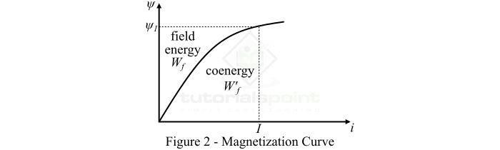
For a linear electromagnetic system, the energy stored in the magnetic field is given by,
$$\mathrm{\mathit{W_{f}}\:=\:\int_{0}^{\mathit{\psi _{\mathrm{1}}}}\mathit{id\psi }\:=\:\int_{0}^{\psi_{\mathrm{1}} }\frac{\psi }{\mathit{L}}\mathit{d\psi }}$$
Where, $\psi\:=\:\mathit{N\phi }\:=\:\mathit{Li}$ and L is the self-inductance of the coil.
$$\mathrm{\therefore \mathit{W_{f}}\:=\:\frac{\psi ^{\mathrm{2}}}{2\mathit{L}}\:=\:\frac{1}{2}\mathit{Li^{\mathrm{2}}}\cdot \cdot \cdot (7)}$$
Concept of Coenergy
Coenergy is an imaginary concept used to derive expressions for torque developed in an electromagnetic system. Thus, the coenergy has no physical significance in the system.
Basically, the coenergy is the area between the $\psi -i$ curve and the current axis and is denoted by $\mathit{W_{f}^{'}}$ as shown above in Figure-2.
Mathematically, the coenergy is given by,
$$\mathrm{\mathit{W_{f}^{'}}\:=\:\int_{0}^{i}\psi \mathit{di}\:=\:\int_{0}^{i}\mathit{Li\:di}}$$
$$\mathrm{\Rightarrow \mathit{W_{f}^{'}}\:=\:\frac{1}{2}\mathit{Li^{\mathrm{2}}}\cdot \cdot \cdot (8)}$$
From equations (7) and (8), it is clear that for a linear magnetic system, the energy stored in the magnetic field and the coenergy are equal.
Singly-Excited and Doubly Excited Systems
Excitation means providing electrical input to an electromechanical energy conversion device such as electric motors. The excitation produces working magnetic field in the electrical machine. Some electrical machines require single electrical input whereas some others require two electrical inputs.
Therefore, depending on the number of electrical inputs to electromechanical energy conversion systems, they can be classified into two types −
Singly-Excited System
Doubly-Excited System
Singly Excited System
As its name implies, a singly-excited system is one which consists of only one electrically energized coil to produce working magnetic field in the machine or any other electromechanical energy conversion device. Hence, the singly-excited system requires only one electrical input.
A singly excited system consists of coil wound around a magnetic core and is connected to a voltage source so that it produces a magnetic field. Due to this magnetic field, the rotor (or moving part) which is made up of ferromagnetic material experiences a torque which move it towards a region where the magnetic field is stronger, i.e., the torque exerted on the rotor tries to position it such that it shows minimum reluctance in the path of magnetic flux. The reluctance depends upon the rotor angle. This torque is known as reluctance torque or saliency torque because it is caused due to saliency of the rotor.
Analysis of Singly Excited System
We made following assumption to analyze the singly-excited system −
For any rotor position, the relationship between flux linkage ($\psi $) and current ($\mathit{i}$) is linear.
The coil has negligible leakage flux, which means all the magnetic flux flows through the main magnetic path.
Hysteresis loss and eddy-current loss are neglected.
All the electric fields are neglected and the magnetic field is predominating.
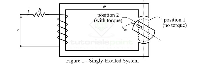
Consider the singly-excited system as shown in Figure-1. If R is the resistance of the coil circuit, the by applying KVL, we can write the voltage equation as,
$$\mathrm{\mathit{v\:=\:iR\:+\:\frac{\mathit{d\psi }}{\mathit{dt}}}\cdot \cdot \cdot (1)}$$
On multiplying equation (1) by current $\mathit{i}$, we have,
$$\mathrm{\mathit{vi\:=\:i^{\mathrm{2}}R\:+\mathit{i}\:\frac{\mathit{d\psi }}{\mathit{dt}}}\cdot \cdot \cdot (2)}$$
We are assuming initial conditions of the system zero and integrating the equation (2) on both side with respect to time, we obtain,
$$\mathrm{\int_{0}^{\mathit{T}}\mathit{vi\:dt}\:=\:\int_{0}^{\mathit{T}}\left ( i^{\mathrm{2}}\mathit{R}\:+\mathit{i}\:\frac{\mathit{d\psi }}{\mathit{dt}} \right )\mathit{dt}}$$
$$\mathrm{\Rightarrow\int_{0}^{\mathit{T}}\mathit{vi\:dt}\:=\:\int_{0}^{\mathit{T}}\mathit{i^{\mathrm{2}}R\:dt}\:+\:\int_{0}^{\psi }\mathit{i\:d\psi }\cdot \cdot \cdot (3)}$$
Equation-3 gives the total electrical energy input the singly-excited system and it is equal to two parts namely,
First part is the electrical loss ($\mathit{W_{el}}$).
Second part is the useful electrical energy which is the sum of field energy ($\mathit{W_{f}}$) and output mechanical energy ($\mathit{W_{m}}$).
Therefore, symbolically we may express the Equation-3 as,
$$\mathrm{\mathit{W_{in}}\:=\:\mathit{W_{el}}\:=\:\left (\mathit{W_{f}} \:+\:\mathit{W_{m}} \right )}\cdot \cdot \cdot (4)$$
The energy stored in the magnetic field of a singly-excited system is given by,
$$\mathrm{\mathit{W_{f}}\:=\: \int_{0}^{\psi }\mathit{i\:d\psi }\:=\:\int_{0}^{\psi }\frac{\psi }{\mathit{L}}\mathit{d\psi }\:=\:\frac{\psi ^{\mathrm{2}}}{2\mathit{L}}\cdot \cdot \cdot (5)}$$
For a rotor movement, where the rotor angle is $\mathit{\theta _{m}}$, the electromagnetic torque developed in the singly-excited system is given by,
$$\mathrm{\mathit{\tau _{e}}\:=\:\frac{\mathit{i^{\mathrm{2}}}}{\mathrm{2}}\frac{\mathit{\partial L}}{\mathit{\partial \theta _{m}}}\cdot \cdot \cdot (6)}$$
The most common examples of singly-excited system are induction motors, PMMC instruments, etc.
Doubly Excited System
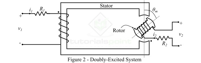
An electromagnetic system is one which has two independent coils to produce magnetic field is known as doubly-excited system. Therefore, a doubly-excited system requires two separate electrical inputs.
Analysis of Doubly Excited System
A doubly-excited system consists of two main parts namely a stator and a rotor as shown in Figure-2. Here, the stator is wound with a coil having a resistance R1 and the rotor is wound with a coil of resistance R2. Therefore, there are two separated windings which are excited by two independent voltage sources.
In order to analyze the double-excited system, the following assumption are made −
For any rotor position the relationship between flux-linkage ($\psi$) and current is linear.
Hysteresis and eddy current losses are neglected.
The coils have negligible leakage flux.
The electric fields are neglected and the magnetic fields are predominating.
The magnetic flux linkages to two windings are given by,
$$\mathrm{\psi _{\mathrm{1}}\:=\:\mathit{L_{\mathrm{1}}i_{\mathrm{1}}}\:+\:\mathit{Mi_{\mathrm{2}}}}\cdot \cdot \cdot (7)$$
$$\mathrm{\psi _{\mathrm{2}}\:=\:\mathit{L_{\mathrm{2}}i_{\mathrm{2}}}\:+\:\mathit{Mi_{\mathrm{2}}}}\cdot \cdot \cdot (8)$$
Where, M is the mutual inductance between two windings.
By applying KVL, we can write the equations of instantaneous voltage for two coils as,
$$\mathrm{\mathit{v}_{\mathrm{1}}\:=\:\mathit{i_{\mathrm{1}}R_{\mathrm{1}}}\:+\:\frac{\mathit{d\psi _{\mathrm{1}}}}{\mathit{dt}}}\cdot \cdot \cdot (9)$$
$$\mathrm{\mathit{v}_{\mathrm{2}}\:=\:\mathit{i_{\mathrm{2}}R_{\mathrm{2}}}\:+\:\frac{\mathit{d\psi _{\mathrm{2}}}}{\mathit{dt}}}\cdot \cdot \cdot (10)$$
In case of doubly-excited system, the energy stored in the magnetic field is given by,
$$\mathrm{\mathit{W_{f}}\:=\:\frac{1}{2}\mathit{L_{\mathrm{1}}i_{\mathrm{1}}^{\mathrm{2}}}\:+\:\frac{1}{2}\mathit{L_{\mathrm{2}}i_{\mathrm{2}}^{\mathrm{2}}}\:+\:\mathit{Mi_{\mathrm{1}}i_{\mathrm{2}}}\cdot \cdot \cdot (11)}$$
And, the electromagnetic torque developed in the doubly excited system is given by,
$$\mathrm{\mathit{\tau _{e}}\:=\:\frac{\mathit{i_{\mathrm{1}}^{\mathrm{2}}}}{\mathrm{2}}\frac{\mathit{dL_{\mathrm{1}}}}{\mathit{d\theta _{m}}}\:+\:\frac{\mathit{i_{\mathrm{2}}^{\mathrm{2}}}}{\mathrm{2}}\frac{\mathit{dL_{\mathrm{2}}}}{\mathit{d\theta _{m}}}\:+\:\mathit{i_{\mathrm{1}}i_{\mathrm{2}}}\frac{\mathit{dM}}{\mathit{d\theta _{m}}}\cdot \cdot \cdot (12)}$$
In Equation-12, the first two terms are the reluctance torque and the last term gives the co-alignment torque due to interaction of two fields.
The practical examples of doubly-excited system are synchronous machines, tachometer, separately-excited DC machines, etc.
Rotating Electrical Machines
Almost all electrical machines have several similar properties and features. The following discussion will explain the basic common features of rotating electrical machines. Where, a rotating electrical machine is one which has a moving (rotating) part, called rotor. The common examples of rotating electrical machines motors and generators.
In a rotating electrical machine, the torque produced can be considered in terms of the instantaneous flux pattern. According to this concept, a torque is produced in an electrical machine when the net magnetic field has asymmetry or distortion.
In any rotating electrical machine, the mechanical forces (torques) are produced due to the following two magnetic field effects −
Alignment of magnetic field lines
Interaction between magnetic fields and current-carrying conductors
In practical electrical machine, magnetic fields are produced by energizing a coil system. It is because, this method of magnetic field production relatively versatile and economic.
Basic Structure of Rotating Electrical Machines
The basic construction and structure of all rotating electrical machines is similar. A typical rotating electrical machine consists of two main parts namely,
Stator
Rotor
The stator and rotor are separated by an air gap. As the name implies, the stator is the stationary (non-movable) part of the electrical machine. In general, the stator is the outer frame of the machine. The rotor is the rotating (movable) part of the machine. Both stator and rotor are constructed by using laminated ferromagnetic materials to reduce the reluctance in the path of magnetic flux.

All rotating electrical machines consist of two windings, one placed on the stator part and another on the rotor part. The winding of the machine in which voltage is induced is known as armature winding. The winding which is used to produce the main working magnetic flux in the machine is known as field winding. Sometimes, instead of field winding, permanent magnets are used to produce the main magnetic flux.
Rotating Magnetic Field
The resultant magnetic field which revolve in the space and is produced by a system of windings (coils) symmetrically placed and supplied with poly-phase currents is known as rotating magnetic field (RMF).
The rotating magnetic field is such as that its magnetic poles do not remain in a fixed position, but go on shifting their positions. The speed of rotation of the magnetic field is known as synchronous speed and is denoted by NS. Mathematically, the synchronous speed is given by,
$$\mathrm{\mathit{N_{s}}\:=\:\frac{120\mathit{f}}{\mathit{P}}}$$
Where, f is the supply frequency in Hz and P is the number of poles. It is measured in RPM (Revolution per Minute).
Machine Torques
Torque is defined as the turning movement of force. The torque is the main factor which rotates the rotor of the machine. In electromechanical devices, there are two types of torques developed −
Electromagnetic Torque
Reluctance Torque
Electromagnetic Torque
The electromagnetic torque is one which produced due to interaction of the magnetic fields produced by the currents in two coils which may move relative to each other. In a rotating electrical machine, under normal operating conditions, there are two magnetic fields present a magnetic field from the stator circuit and another magnetic field from the rotor circuit. The interaction between these two magnetic fields produces the torque in the machine. This torque is known as electromagnetic torque. The electromagnetic torque is also known as induced torque.
Reluctance Torque
When an object made up of a ferromagnetic material is placed in an external magnetic field experiences a force (torque) which causes the object to align it with the external magnetic field, it is known as reluctance torque.
The reluctance torque occurs because the external magnetic field induced an internal magnetic field in the ferromagnetic object, and a torque is produced by interaction of the two magnetic fields moving the object to align with the external magnetic field. Since, the reluctance torque on the object tries to position it to give minimum reluctance (or saliency) for the magnetic flux. Therefore, the reluctance torque is also known as alignment torque or saliency torque.
Faradays Laws of Electromagnetic Induction
When a changing magnetic field links to a conductor or coil, an EMF is produced in the conductor or coil, this phenomenon is known as electromagnetic induction. The electromagnetic induction is the most fundamental concept used to design the electrical machines.
Michael Faraday, an English scientist, performed several experiments to demonstrate the phenomenon of electromagnetic induction. He concluded the results of all experiments into two laws, popularly known as Faradays laws of electromagnetic induction.
Faradays First Law
Faradays first law of electromagnetic induction provides information about the condition under which an EMF is induced in a conductor or coil. The first law states that −
When a magnetic flux linking to a conductor or coil changes, an EMF is induced in the conductor or coil.
Therefore, the basic need for inducing EMF in a conductor or coil is the change in the magnetic flux linking to the conductor or coil.
Faradays Second Law
Faradays second law of electromagnetic induction gives the magnitude of the induced EMF in a conductor or coil and it may be states as follows −
The magnitude of the induced EMF in a conductor or coil is directly proportional to the time rate of change of magnetic flux linkage.
Explanation
Consider a coil has N turns and magnetic flux linking the coil changes from $\mathit{\phi _{\mathrm{1}}}$ weber to $\mathit{\phi _{\mathrm{2}}}$ weber in time t seconds. Now, the magnetic flux linkage ($\mathit{\psi }$) to a coil is the product of magnetic flux and number of turns in the coil. Therefore,
$$\mathrm{\mathrm{Initial\: magnetic\: flux\: linkage,}\mathit{\psi _{\mathrm{1}}}\:=\:\mathit{N\phi _{\mathrm{1}}}}$$
$$\mathrm{\mathrm{Final\: magnetic\: flux\: linkage,}\mathit{\psi _{\mathrm{2}}}\:=\:\mathit{N\phi _{\mathrm{2}}}}$$
According to Faradays law of electromagnetic induction,
$$\mathrm{\mathrm{Induced\: EMF,}\mathit{e}\propto \frac{\mathit{N\phi _{\mathrm{2}}}-\mathit{N\phi} _{\mathrm{1}}}{\mathit{t}}\cdot \cdot \cdot (1)}$$
$$\mathrm{\Rightarrow \mathit{e}\:=\:\mathit{k}\left ( \frac{\mathit{N\phi _{\mathrm{2}}}-\mathit{N\phi} _{\mathrm{1}}}{\mathit{t}} \right )}$$
Where, k is a constant of proportionality, its value is unity in SI units.
Therefore, the induced EMF in the coil is given by,
$$\mathrm{\mathit{e}\:=\:\frac{\mathit{N\phi _{\mathrm{2}}}-\mathit{N\phi} _{\mathrm{1}}}{\mathit{t}}\cdot \cdot \cdot (2)}$$
In differential form,
$$\mathrm{\mathit{e}\:=\:\mathit{N}\frac{\mathit{d\phi }}{\mathit{dt}}\cdot \cdot \cdot (3)}$$
The direction of induced EMF is always such that it tends set up a current which produces a magnetic flux that opposes the change of magnetic flux responsible for inducing the EMF. Therefore, the magnitude and direction of the induced EMF in the coil is to be written as,
$$\mathrm{ \mathit{e}\:=\:\mathit{-N}\frac{\mathit{d\phi }}{\mathit{dt}}\cdot \cdot \cdot (4)}$$
Where, the negative (-) sign shows that the direction of the induced EMF is such that it opposes the cause that produces it, i.e., the change in the magnetic flux, this statement is known as Lenzs law. The equation (4) is the mathematical representation of Lenzs law.
Concept of Induced EMF
According to principle of electromagnetic induction, when the magnetic flux linking to a conductor or coil changes, an EMF is induced in the conductor or coil. In practice, the following two ways are used to bring the change in the magnetic flux linkage.
Method 1 − Conductor is moving in a stationary magnetic field
We can move a conductor or coil in a stationary magnetic field in such a way that the magnetic flux linking to the conductor or coil changes in magnitude. Consequently, an EMF is induced in the conductor. This induced EMF is known as dynamically induced EMF. It is so called because the EMF induced in a conductor which is in motion. Example of dynamically induced EMF is the EMF generated in the AC and DC generators.
Method 2 − A stationary conductor is placed in a changing magnetic field
When a stationary conductor or coil is placed in a moving or changing magnetic field, an EMF is induced in the conductor or coil. The EMF induced in this way is known as statically induced EMF. It is so called because the EMF is induced in a conductor which is stationary. The EMF induced in a transformer is an example of statically induced EMF.
Therefore, from the discussion, it is clear that the induced EMF can be classified into two major types namely,
Dynamically Induced EMF
Statically Induced EMF
Dynamically Induced EMF
As discussed in the above section that the dynamically induced EMF is one which induced in a moving conductor or coil placed in a stationary magnetic field. The expression for the dynamically induced EMF can be derived as follows −
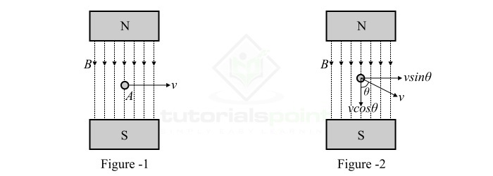
Consider a single conductor of length l meters located in a uniform magnetic field of magnetic flux density B Wb/m2 as shown in Figure-1. This conductor is moving at right angles relative to the magnetic field with a velocity of v m/s.
Now, if the conductor moves through a small distance dx in time dt seconds, then the area swept by the conductor is given by,
$$\mathrm{\mathit{A\:=\:l\times dx\:}\mathrm{m^{\mathrm{2}}}}$$
Therefore, the magnetic flux cut by the conductor is given by,
$$\mathrm{\mathit{d\phi }\:=\:\mathrm{Flux\:density\times Area\: swept}}$$
$$\mathrm{\Rightarrow \mathit{d\phi }\:=\:\mathit{B\times l\times dx}\:\mathrm{Wb}}$$
According to Faradays law of electromagnetic induction, the EMF induced in the conductor is given by,
$$\mathrm{\mathit{e}\:=\:\mathit{N}\frac{\mathit{d\phi }}{\mathit{dt}}\:=\:\mathit{N}\frac{\mathit{Bldx}}{\mathit{dt}}}$$
Since, we have taken only a single conductor, thus N = 1.
$$\mathrm{\mathit{e}\:=\:\mathit{Blv}\:\mathrm{volts}\cdot \cdot \cdot (1)}$$
Where, v = dx/dt, velocity of the conductor in the magnetic field.
If there is angular motion of the conductor in the magnetic field and the conductor moves at an angle relative to the magnetic field as shown in Figure-2. Then, the velocity at which the conductor moves across the magnetic field is equal to "vsinθ". Thus, the induced EMF is given by,
$$\mathrm{\mathit{e}\:=\:\mathit{B\:l\:v}\:\mathrm{sin\mathit{\theta }}\:\mathrm{volts}\cdot \cdot \cdot (2)}$$
Statically Induced EMF
When a stationary conductor is placed in a changing magnetic field, the induced EMF in the conductor is known as statically induced EMF. The statically induced EMF is further classified into following two types −
Self-Induced EMF
Mutually Induced EMF
Self Induced EMF
When EMF is induced in a conductor or coil due to change of its own magnetic flux linkage, it is known as self-induced EMF.

Consider a coil of N turn as shown in Figure-3. The current flowing through the coil establishes a magnetic field in the coil. If the current in the coil changes, then the magnetic flux linking the coil also changes. This changing magnetic field induces an EMF in the coil according to the Faradays law of electromagnetic induction. This EMF is known as self-induced EMF and the magnitude of the self-induced EMF is given by,
$$\mathrm{\mathit{e}\:=\:\mathit{N}\frac{\mathit{d\phi }}{\mathit{dt}}}$$
Mutually Induced EMF
The EMF induced in a coil due to the changing magnetic field of a neighboring coil is known as mutually induced EMF.
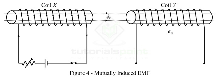
Consider two coils X and Y placed adjacent to each other as shown in Figure-4. Here, a fraction of the magnetic flux produced by the coil X links with the coil Y. This magnetic flux of coil X which is common to both coils X and Y is known as mutual flux ($\mathit{\phi _{m}}$).
If the current in coil X is changed, then the mutual flux also changes and hence EMF is induced in both the coils. Where, the EMF induced in coil X is known as self-induced EMF and the EMF induced in coil Y is called mutually induced EMF.
According to Faradays law, the magnitude of the mutually induced EMF is given by,
$$\mathrm{\mathit{e_{m}}\:=\:\mathit{N_{Y}}\frac{\mathit{d\phi _{m}}}{\mathit{dt}}}$$
Where,$\mathit{N_{Y}}$ is the number of turns in coil Y and $\frac{\mathit{d\phi _{m}}}{\mathit{dt}}$ is rate of change of mutual flux.
Flemings Left Hand and Right Hand Rules
All electrical machines work on the principle of electromagnetic induction. According to this principle, if there is relative motion between a conductor and a magnetic field, then an EMF is induced in the conductor. On the other hand, if a current carrying conductor is placed in a magnetic field, the conductor experiences a force. For practical and analytical purposes, it is important to determine the direction of induced EMF and force acting on the conductor. Flemings hand rules are used for that.
An English electrical engineer and physicist John Ambrose Fleming stated two rules in late 19th century to determine the direction of induced EMF and force acting on a current carrying conductor placed in a magnetic field. These rules popularly known as Flemings Left Hand Rule and Flemings Right Hand Rule.
Basically, both left hand rule and right hand rule show a relationship between magnetic field, force and current.
Flemings left hand rule is used to determine the direction of force acting on a current carrying conductor when it placed in a magnetic field, hence it is mainly applicable in electric motors. Whereas, Flemings right hand rule is used to determine the direction of induced EMF in a conductor moving relative to a magnetic field, thus it is mainly applicable in electric generators.
Flemings Left Hand Rule
Flemings left hand rule is particularly suitable to find the direction of force on a current carrying conductor in a magnetic field and it may be stated as under −
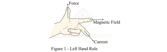
Stretch out the forefinger, middle finger and thumb of your left hand so that they are at right angles (perpendicular) to one another as shown in figure 1. If the forefinger points in the direction of magnetic field, middle finger in the direction of current in the conductor, then the thumb will point in the direction of force on the conductor.
In practice, Flemings left hand rule is applied to determine the direction of motion of conductor in electric motors.
Flemings Right Hand Rule
Flemings right hand rule is particularly suitable to determine the direction of induced EMF and hence electric current in a conductor when there is a relative motion between the conductor and magnetic field. Flemings left hand rule may be stated as under −
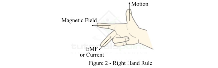
Stretch out the forefinger, middle finger and thumb of your right hand so that they are at right angles (perpendicular) to one another as shown in figure 2. If the forefinger points in the direction of magnetic field, thumb in the direction of motion of the conductor, then the middle finger will point in the direction of induced EMF or current.
In practice, Flemings right hand rule is used to determine the direction of induced EMF and current in the electric generators.
Comparison of Flemings Left Hand Rule and Right Hand Rule
The following table gives a brief comparison of Flemings left hand and right hand rules −
| Parameters | Flemings Left Hand Rule | Flemings Right Hand Rule |
|---|---|---|
| Purpose | Flemings LHR is used to determine the direction of force acting on a current carrying conductor in a magnetic field. | Flemings RHR is used to find the direction of induced EMF or current in a conductor. |
| Use | Flemings left hand rule is mainly applicable in electric motors. | Flemings right hand rule is applicable in electric generators. |
Electrical Transformer
In electrical and electronic systems, the electrical transformer is one of the most useful electrical machine. An electrical transformer can increase or decrease the magnitude of alternating voltage or current. It is the major reason behind the widespread use of alternating currents rather than direct current. A transformer does not have any moving part. Therefore, it has very high efficiency up to 99% and very strong and durable construction.
Electrical Transformer
A transformer or electrical transformer is a static AC electrical machine which changes the level of alternating voltage or alternating current without changing in the frequency of the supply.
A typical transformer consists of two windings namely primary winding and secondary winding. These two windings are interlinked by a common magnetic circuit for transferring electrical energy between them.
Principle of Transformer Operation
The operation of the transformer is based on the principle of mutual inductance, which states that when a changing magnetic field of one coil links to another coil, an EMF is induced in the second coil.
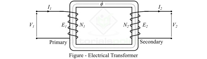
When an alternating voltage V1 is applied to the primary winding, an alternating current flows through it and produces an alternating magnetic flux. This changing magnetic flux flows through the core of the transformer and links to the secondary winding. According to Faradays law of electromagnetic induction, an EMF E2 is induced in the secondary winding due to the linkage of changing magnetic flux of the primary winding. If the secondary winding circuit is closed by connecting a load, then this induced EMF E2 in the secondary winding causes a secondary current I2 to flow through the load.
Although the changing magnetic flux of primary winding is also linked with the primary winding itself. Hence, an EMF E1 is induced in the primary winding due to its own inductance effect. The value of E1 and E2 can be given by the following formulae,
$$\mathrm{\mathit{E_{\mathrm{1}}}\:=\:-\mathit{N_{\mathrm{1}}}\frac{\mathit{d\phi }}{\mathit{dt}}}$$
$$\mathrm{\mathit{E_{\mathrm{2}}}\:=\:-\mathit{N_{\mathrm{2}}}\frac{\mathit{d\phi }}{\mathit{dt}}}$$
Where N1 and N2 are the number of turns in the primary winding and secondary winding respectively.
On taking the ratio of E2 and E2, we get,
$$\mathrm{\frac{\mathit{E_{\mathrm{2}}}}{\mathit{E_{\mathrm{1}}}}\:=\:\frac{\mathit{N_{\mathrm{2}}}}{\mathit{N_{\mathrm{1}}}}}$$
This expression is known as transformation ratio of the transformer. The transformation ratio depends on the number of turns in primary and secondary windings. Which means the magnitude of output voltage depends on the relative number of turns in primary and secondary windings.
If N2 > N1, then E2 > E2, i.e., the output voltage of the transformer is more than the input voltage, and such a transformer is known as set-up transformer. On the other hand, if N1 > N2, then E1 > E2 i.e., the output voltage is less than input voltage, such a transformer is called step-down transformer.
From the circuit diagram of the transformer, we can see that there is no electrical connection between the primary and secondary instead they are linked with the help of a magnetic field. Thus, a transformer enables us to transfer AC electrical power magnetically from one circuit to another which a change in the voltage and current level.
Important Points
Note the following important points about transformers −
The operation of transformer is based on the principle of electromagnetic induction.
The transformer does not change the frequency, i.e. the frequency of input supply and output supply remains the same.
Transformer is a static electrical machine, which means it does not have any moving part. Hence, it has very high efficiency.
Transformer cannot work with direct current because it is an electromagnetic induction machine.
There is no direct electrical connection between primary and secondary windings. The AC power is transferred from primary to secondary through magnetic flux.
Construction of Transformer
A transformer consists of three major parts namely a primary winding, a secondary winding and a magnetic core. The primary winding is one that used to input the supply and secondary winding is one that used to take output. The magnetic core is used to confine the magnetic flux to a definite path.
We design a transformer in such a way that it approaches the characteristics of an ideal transformer. In practice, we incorporate the following design features for transformer construction −
The core of the transformer is made up of high grade silicon steel which has high permeability and low hysteresis loss.
The core is laminated to minimize the eddy current loss.
It is a usual and more efficient practice to wind one-half of the primary and secondary windings on one limb instead of placing primary on one limb and secondary on the other. This ensures tight magnetic coupling between the two windings and hence reduces the leakage flux considerably.
The winding resistances R1 and R2 are reduced as much as possible so that they cause lowest I2R loss and temperature rise and ensure higher efficiency.
Transformer Construction
A transformer can be constructed in the following two ways −
Core Type Transformer Construction
Shell Type Transformer Construction
Core Type Construction of Transformer
In the core type construction of the transformer, the magnetic core has two vertical lags (called limbs) and two horizontal sections (called yokes). The half of the primary winding and the half of the secondary winding are placed around each limb as shown in Figure-1.
This arrangement of windings minimizes the leakage flux. In practice, the low-voltage winding (it could be primary or secondary) is placed next to the core and the high-voltage winding is placed around the low-voltage winding. This considerably reduces the requirement of insulating material.
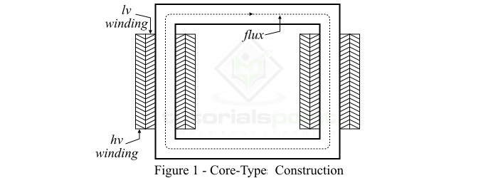
The main advantage of the core-type construction of transformers is that it is easier to dismantle for repair and maintenance. The core-type construction is most suitable for high-voltage and high-power transformers because in the core type construction, the nature cooling is more efficient.
Shell Type Construction of Transformer
In the shell-type construction of transformers, both primary and secondary windings are wound on the central limb, while the two outer limbs complete the low reluctance flux paths as shown in Figure-2.
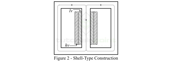
In this case, each winding is sub-divided into sections, and the low-voltage (lv) winding sections and high-voltage (hv) winding sections are alternatively put in the form of a sandwich. Therefore, this type of winding is also called as sandwich winding or disc winding.
The shell-type construction of transformers provides better mechanical support against electromagnetic forces between the current-carrying windings. Also, this transformer construction provides a shorter path for magnetic flux and hence requires small magnetizing current. The shell-type construction is more suitable for low voltage transformers because of poor nature cooling due to the embedding of the windings.
EMF Equation of Transformer
For electrical transformer, the EMF equation is a mathematical expression used to find the magnitude of induced EMF in the windings of the transformer.
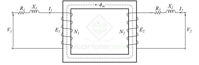
Consider a transformer as shown in the figure. If N1 and N2 are the number of turns in primary and secondary windings. When we apply an alternating voltage V1 of frequency f to the primary winding, an alternating magnetic flux $\phi$ is produced by the primary winding in the core.

If we assume sinusoidal AC voltage, then the magnetic flux can be given by,
$$\mathrm{\mathit{\phi }\:=\:\phi _{m}\:\mathrm{sin}\:\mathit{\omega t}\:\cdot \cdot \cdot (1)}$$
Now, according to principle of electromagnetic induction, the instantaneous value of EMF e1 induced in the primary winding is given by,
$$\mathrm{\mathit{e_{\mathrm{1}}}\:=\:\mathit{-N_{\mathrm{1}}}\frac{\mathit{d\phi }}{\mathit{dt}}}$$
$$\mathrm{\Rightarrow \mathit{e_{\mathrm{1}}}\:=\:\mathit{-N_{\mathrm{1}}}\frac{\mathit{d}}{\mathit{dt}}\left ( \phi _{m}\: \mathrm{sin}\:\mathit{\omega t}\right )}$$
$$\mathrm{\Rightarrow \mathit{e_{\mathrm{1}}}\:=\:\mathit{-N_{\mathrm{1}}}\:\mathit{\omega \phi \:cos\:\omega t}}$$
$$\mathrm{\Rightarrow \mathit{e_{\mathrm{1}}}\:=\:-\mathrm{2}\mathit{\pi fN_{\mathrm{1}}}\:\mathit{\phi_{m} \:cos\:\omega t}}$$
Where,
$$\mathrm{\mathit{\omega \:=\:\mathrm{2}\pi f}}$$
$$\mathrm{\because -\mathit{cos\:\omega t}\:=\:\mathrm{sin}\left ( \mathit{\omega t-\mathrm{90^{\circ}}} \right )}$$
Therefore,
$$\mathrm{\mathit{e_{\mathrm{1}}}\:=\:\mathrm{2}\mathit{\phi fN_{\mathrm{1}}}\:\mathit{\phi_{m}\:\mathrm{sin}\left ( \mathit{\omega t-\mathrm{90^{\circ}}} \right )}}\:\cdot \cdot \cdot (2)$$
Equation (2) may be written as,
$$\mathrm{\mathit{e_{\mathrm{1}}}\:=\:\mathit{E_{m_{\mathrm{1}}}}\mathrm{sin}\left ( \mathit{\omega t-\mathrm{90^{\circ}}} \right )\:\cdot \cdot \cdot (3)}$$
Where,$\mathit{E_{m_{\mathrm{1}}}}$ is the maximum value of induced EMF $\mathit{e_{\mathrm{1}}}$.
$$\mathrm{\mathit{E_{\mathrm{m1}}}\:=\:\mathrm{2}\mathit{\pi fN_{\mathrm{1}}}\:\mathit{\phi_{m}}}$$
Now, for sinusoidal supply, the RMS value $\mathit{E_{\mathrm{1}}}$ of the primary winding EMF is given by,
$$\mathrm{\mathit{E_{\mathrm{1}}}\:=\:\frac{\mathit{E_{m\mathrm{1}}}}{\sqrt{2}}\:=\:\frac{2\mathit{\pi fN_{\mathrm{1}}}\phi_{m}}{\sqrt{2}}}$$
$$\mathrm{\therefore\mathit{E_{\mathrm{1}}}\:=\:4.44\:\mathit{f\phi _{m}N_{\mathrm{1}}}\:\cdot \cdot \cdot (4)}$$
Similarly, the RMS value E2 of the secondary winding EMF is,
$$\mathrm{\mathit{E_{\mathrm{2}}}\:=\:4.44\:\mathit{f\phi _{m}N_{\mathrm{2}}}\:\cdot \cdot \cdot (5)}$$
In general,
$$\mathrm{\mathit{E}\:=\:4.44\:\mathit{f\phi _{m}N}\:\cdot \cdot \cdot (6)}$$
Equation (6) is known as EMF equation of a transformer.
For a given transformer, if we divide the EMF equation by the supply frequency, we get,
$$\mathrm{\frac{\mathit{E}}{\mathit{f}}\:=\:4.44\:\phi _{m}\mathit{N}\:=\:\mathrm{Constant}}$$
Which means the induced EMF per unit frequency is constant but it is not same on both primary and secondary side of the given transformer.
Also, from equations (4) and (5), we have,
$$\mathrm{\frac{\mathit{E_{\mathrm{1}}}}{\mathit{E_{\mathrm{2}}}}\:=\:\frac{\mathit{N_{\mathrm{1}}}}{\mathit{N_{\mathrm{2}}}}\:or\:\frac{\mathit{E_{\mathrm{1}}}}{\mathit{N_{\mathrm{1}}}}\:=\:\frac{\mathit{E_{\mathrm{2}}}}{\mathit{N_{\mathrm{2}}}}}$$
Hence, in a transformer, the induced EMF per turn in the primary winding is equal to the induced EMF per turn in the secondary winding.
Numerical Example
A single phase 3300/240 V, 50 Hz transformer has a maximum magnetic flux of 0.0315 Wb in the core. Calculate the number of turns in primary and secondary windings.
Solution
Given data,
$$\mathrm{\mathit{E_{\mathrm{1}}\:=\:\mathrm{3300}\:\mathrm{V}\:\mathrm{and}\:\mathit{E_{\mathrm{2}}\:=\:\mathrm{240}\:V}}}$$
$$\mathrm{\mathit{f}\:=\:50\:Hz;\:\phi _{m}\:=\:0.0315\:Wb}$$
The EMF equation of the transformer is,
$$\mathrm{\mathit{E}\:=\:4.44\:\mathit{f\phi _{m}N}}$$
Therefore, for primary winding,
$$\mathrm{\mathit{N_{\mathrm{1}}}\:=\:\frac{\mathit{E_{\mathrm{1}}}}{4.44\:\mathit{f\phi _{m}}}\:=\:\frac{3300}{4.44\times 50\times 0.0315}}$$
$$\mathrm{\mathit{N_{\mathrm{1}}}\:=\:471.9\:=\:472}$$
Also, for secondary winding,
$$\mathrm{\mathit{N_{\mathrm{2}}}\:=\:\frac{\mathit{E_{\mathrm{2}}}}{4.44\:\mathit{f\phi _{m}}}\:=\:\frac{240}{4.44\times 50\times 0.0315}}$$
$$\mathrm{\mathit{N_{\mathrm{2}}}\:=\:34.32\:=\:35}$$
It is not possible for a winding to have part of a turn. Thus, the number of turns should be a whole number.
Turns Ratio and Voltage Transformation Ratio
As discussed in the previous chapter, the EMF of equation of a transformer is given by,
$$\mathrm{\mathit{E}\:=\:4.44\:\mathit{f\phi _{m}\:N}}$$
For primary winding,
$$\mathrm{\mathit{E_{\mathrm{1}}}\:=\:4.44\:\mathit{f\phi _{m}\:N_{\mathrm{1}}}\:\cdot \cdot \cdot (1)}$$
For secondary winding,
$$\mathrm{\mathit{E_{\mathrm{2}}}\:=\:4.44\:\mathit{f\phi _{m}\:N_{\mathrm{2}}}\:\cdot \cdot \cdot (2)}$$
Turns Ratio of Transformer
From equations (1) and (2), we have,
$$\mathrm{\frac{\mathit{E_{\mathrm{1}}}}{\mathit{E_{\mathrm{2}}}}\:=\:\frac{\mathit{N_{\mathrm{1}}}}{\mathit{N_{\mathrm{2}}}}\:=\mathrm{a}\:\:\cdot \cdot \cdot (3)}$$
The constant "a" is known as the turns ratio of the transformer. It may be defined as under,
The ratio of number of turns in the primary winding the number of turns in the secondary winding of a transformer is known as turns ratio.
Voltage Transformation Ratio of Transformer
The ratio of output voltage to the input voltage of transformer is known as voltage transformer ratio, i.e.,
$$\mathrm{\mathrm{Transformation\: Ratio}\:=\:\frac{Output \:Voltage}{Input \:Voltage}}$$
Thus, if V1 is the input voltage and V2 is the output voltage of a transformer, then its transformation ratio is given by,
$$\mathrm{\mathrm{Transformation\: Ratio}\:=\:\frac{\mathit{V_{\mathrm{2}}}}{\mathit{V_{\mathrm{1}}}}\:\cdot \cdot \cdot (4)}$$
For an ideal transformer, V1 = E1 and V2 = E2, then
$$\mathrm{\mathrm{Transformation\: Ratio}\:=\:\frac{\mathit{V_{\mathrm{2}}}}{\mathit{V_{\mathrm{1}}}}\:=\:\frac{\mathit{E_{\mathrm{2}}}}{\mathit{E_{\mathrm{1}}}}\:=\:\:\frac{\mathit{N_{\mathrm{2}}}}{\mathit{N_{\mathrm{1}}}}\:=\:\frac{1}{a}\cdot \cdot \cdot (5)}$$
However, in a practical transformer, there is a small difference between V1 and E1, and V2 and E2, due to winding resistances. Although, this difference is very small so for analysis purposes, we take V1 = E1 and V2 = E2.
Numerical Example (1)
A transformer with 1000 primary turns and 400 secondary turns is supplied from a 220 V AC supply. Calculate the secondary voltage and the volts per turn.
Solution
Given data,
$$\mathrm{\mathit{N_{\mathrm{1}}}\:=\:1000\:\mathrm{and}\:\mathit{N_{\mathrm{2}}}\:=\:400}$$
$$\mathrm{\mathit{V_{\mathrm{1}}}\:=\:220\:V}$$
The turns ratio of transformer is,
$$\mathrm{\frac{\mathit{V_{\mathrm{1}}}}{\mathit{V_{\mathrm{2}}}}\:=\:\frac{\mathit{N_{\mathrm{1}}}}{\mathit{N_{\mathrm{2}}}}}$$
$$\mathrm{\Rightarrow \mathit{V_{\mathrm{2}}}\:=\:\mathit{V_{\mathrm{1}}}\times \frac{\mathit{N_{\mathrm{2}}}}{\mathit{N_{\mathrm{1}}}}\:=\:220\times \frac{400}{1000}}$$
$$\mathrm{\therefore\mathit{V_{\mathrm{2}}}\:=\:88\:\mathrm{Volts}}$$
The volts per turn is given by,
$$\mathrm{\mathrm{For\: primary\: winding}\:=\:\frac{\mathit{V_{\mathrm{1}}}}{\mathit{N_{\mathrm{1}}}}\:=\:\frac{200}{1000}\:=\:0.22\:\mathrm{Volts}}$$
$$\mathrm{\mathrm{For\: Secondary\: winding}\:=\:\frac{\mathit{V_{\mathrm{2}}}}{\mathit{N_{\mathrm{2}}}}\:=\:\frac{88}{400}\:=\:0.22\:\mathrm{Volts}}$$
Hence, from this example, it is clear that the volts per turn for a transformer remain the same on both primary and secondary windings.
Numerical Example (2)
A transformer with an output voltage of 2200 V is supplied at 220 V. If the secondary winding has 2000 turns, then calculate the number of turns in primary winding.
Solution
Given data,
$$\mathrm{\mathit{V_{\mathrm{1}}}\:=\:200\:\mathit{V}\:\mathrm{and}\:\mathit{V_{\mathrm{2}}}\:=\:2200\:\mathit{V}}$$
$$\mathrm{\mathit{N_{\mathrm{2}}}\:=\:2000\:\mathrm{turns}}$$
The turns ratio of transformer is,
$$\mathrm{\frac{\mathit{V_{\mathrm{1}}}}{\mathit{V_{\mathrm{2}}}}\:=\:\frac{\mathit{N_{\mathrm{1}}}}{\mathit{N_{\mathrm{2}}}}}$$
$$\mathrm{\Rightarrow {\mathit{N_{\mathrm{1}}}}\:=\:\mathit{N_{\mathrm{2}}}\:\times \:\frac{\mathit{V_{\mathrm{1}}}}{\mathit{V_{\mathrm{2}}}}\:=\:\mathrm{2000}\:\times \:\frac{220}{2200}\:=\:\mathrm{200\:turns}}$$
Ideal and Practical Transformers
Ideal Transformer
An ideal transformer is an imaginary model of the transformer which possesses the following characteristics −
The primary and secondary windings have negligible (or zero) resistance.
It has no leakage flux, i.e., whole of the flux flows through the magnetic core of the transformer.
The magnetic core has infinite permeability, which means it requires negligible MMF to establish flux in the core.
There are no losses due winding resistances, hysteresis and eddy currents. Hence, its efficiency is 100 %.
Working of an Ideal Transformer
We may analyze the operation of an ideal transformer either on no-load or on-load, which is discussed in the following sections.
Ideal Transformer on No-Load
Consider an ideal transformer on no-load, i.e., its secondary winding is open circuited, as shown in Figure-1. And, the primary winding is a coil of pure inductance.
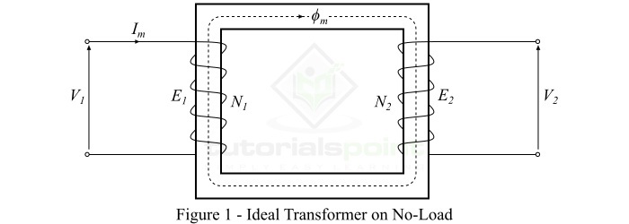
When an alternating voltage $\mathit{V_{\mathrm{1}}}$ is applied to the primary winding, it draws a very small magnetizing current $\mathit{I_{\mathit{m}}}$ to establish flux in the core, which lags behind the applied voltage by 90. The magnetizing current Im produces an alternating flux $\mathit{\phi_{m}}$ in the core which is proportional to and in phase with it. This alternating flux ($\mathit{\phi_{m}}$) links the primary and secondary windings magnetically and induces an EMF $\mathit{E_{\mathrm{1}}}$ in the primary winding and an EMF $\mathit{E_{\mathrm{2}}}$ in the secondary winding.
The EMF induced in the primary winding $\mathit{E_{\mathrm{1}}}$ is equal to and opposite of the applied voltage $\mathit{V_{\mathrm{1}}}$ (according to Lenzs law). The EMFs $\mathit{E_{\mathrm{1}}}$ and $\mathit{E_{\mathrm{2}}}$ lag behind the flux ($\mathit{\phi_{m}}$) by 90, however their magnitudes depend upon the number of turns in the primary and secondary windings. Also, the EMFs $\mathit{E_{\mathrm{1}}}$ and $\mathit{E_{\mathrm{2}}}$ are in phase with each other, while $\mathit{E_{\mathrm{1}}}$ is equal to $\mathit{V_{\mathrm{1}}}$ and 180 out of phase with it.
Ideal Transformer on On-Load
When a load is connected across terminals of the secondary winding of the ideal transformer, the transformer is said to be loaded and a load current flows through the secondary winding and load.
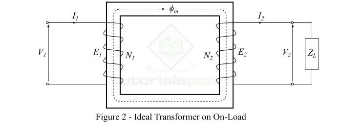
Consider an inductive load of impedance connected across the secondary winding of the ideal transformer as shown in Figure-2. Then, the secondary winding EMF $\mathit{E_{\mathrm{2}}}$ will cause a current $\mathit{I_{\mathrm{2}}}$ to flow through the secondary winding and load, which is given by,
$$\mathrm{\mathit{I_{\mathrm{2}}}\:=\:\frac{\mathit{E_{\mathrm{2}}}}{\mathit{Z_{\mathit{L}}}}\:=\:\frac{\mathit{V_{\mathrm{2}}}}{\mathit{Z_{\mathit{L}}}}}$$
Where, for an ideal transformer, the secondary winding EMF $\mathit{E_{\mathrm{2}}}$ is equal to the secondary winding terminal voltage $\mathit{V_{\mathrm{2}}}$.
Since we considered an inductive load, therefore, the current $\mathit{I_{\mathrm{2}}}$ will lag behind $\mathit{E_{\mathrm{2}}}$ or $\mathit{V_{\mathrm{2}}}$ by an angle of $\mathit{\phi_{\mathrm{2}}}$. Also, the no-load current $\mathit{I_{\mathrm{0}}}$ being neglected because the transformer is ideal one.
The current flowing in the secondary winding ($\mathit{I_{\mathrm{2}}}$) sets up an MMF ($\mathit{I_{\mathrm{2}}}\mathit{N_{\mathrm{2}}}$) which produces a flux $\mathit{\phi_{\mathrm{2}}}$ in opposite direction to the main flux ($\mathit{\phi_{\mathit{m}}}$). As a result, the total flux in the core changes from its original value, however, the flux in the core should not change from its original value. Therefore, to maintain the flux in the core at its original value, the primary current must develop an MMF which can counter-balance the demagnetizing effect of the secondary MMF $\mathit{I_{\mathrm{2}}}\mathit{N_{\mathrm{2}}}$.
Hence, the primary current $\mathit{I_{\mathrm{1}}}$ must flow so that
$$\mathrm{\mathit{I_{\mathrm{1}}}\mathit{N_{\mathrm{1}}}\:=\:\mathit{I_{\mathrm{2}}}\mathit{N_{\mathrm{2}}}}$$
Therefore, the primary winding must draw enough current to neutralize the demagnetizing effect of the secondary current so that the main flux in the core remains constant. Hence, when the secondary current ($\mathit{I_{\mathrm{2}}}$) increases, the primary current ($\mathit{I_{\mathrm{1}}}$) also increases in the same manner and keeps the mutual flux ($\mathit{\phi_{\mathit{m}}}$) constant.
In an ideal transformer on-load, the secondary current $\mathit{I_{\mathrm{2}}}$ lags behind the secondary terminal voltage $\mathit{V_{\mathrm{2}}}$ by an angle of $\mathit{\phi _{\mathrm{2}}}$.
Practical Transformer
A practical transformer is one which possesses the following characteristics −
The primary and secondary windings have finite resistance.
There is a leakage flux, i.e., whole of the flux is not confined to the magnetic core.
The magnetic core has finite permeability, hence a considerable amount of MMF is require to establish flux in the core.
There are losses in the transformer due to winding resistances, hysteresis and eddy currents. Therefore, the efficiency of a practical transformer is always less than 100 %.
The analytical model of a typical practical transformer is shown in Figure-3.
Characteristics of a Practical Transformer
Following are the important characteristics of a Practical Transformer −
Winding Resistances
The windings of a transformer are usually made up of copper conductors. Therefore, both the primary and secondary windings will have winding resistances, which produce the copper loss or $\mathit{i^{\mathrm{2}} \mathit{R}}$ loss in the transformer. The primary winding resistance $\mathit{R_{\mathrm{1}}}$ and the secondary winding resistance $\mathit{R_{\mathrm{2}}}$ act in series with the respective windings as shown in Figure-3.
Iron Losses or Core Losses
The core of the transformer is subjected to the alternating magnetic flux, hence the eddy current loss and hysteresis loss occur in the core. The hysteresis loss and eddy current loss together are known as iron loss or core loss. The iron loss of the transformer depends upon the supply frequency, maximum flux density in the core, volume of the core and thickness of the laminations etc. In a practical transformer, the magnitude of iron loss is practically constant and very small.
Leakage Flux
The current through the primary winding produces a magnetic flux. The flux $\mathit{\phi _{\mathit{m}}}$ which links both primary and secondary windings is the useful flux and is known as mutual flux. However, a fraction of the flux ($\mathit{\phi _{\mathrm{1}}}$) produced by the primary current does not link with the secondary winding.
When a load is connected across the secondary winding, a current flows through it and produces a flux ($\mathit{\phi _{\mathrm{2}}}$), which links only with the secondary winding. Thus, the part of $\mathit{\phi _{\mathrm{1}}}$, and the flux $\mathit{\phi _{\mathrm{2}}}$ that link only their respective winding are known as leakage flux.
The leakage flux has its path through the air which has very high reluctance. Therefore, the effect of primary leakage flux ($\mathit{\phi _{\mathrm{1}}}$) is to introduce an inductive reactance ($ \mathit{X_{\mathrm{1}}}$) in series with the primary winding. Similarly, the secondary leakage flux ($\mathit{\phi _{\mathrm{2}}}$) introduces an inductive reactance ($ \mathit{X_{\mathrm{2}}}$) in series with the secondary winding as shown in Figure-3.
However, the leakage flux in a practical transformer is very small (about 5% of $\mathit{\phi _{m}}$), yet it cannot be ignored. Because the leakage flux paths are through the air, which has very high reluctance. Thus, it requires considerable MMF.
Finite Permeability of Core Material
In general, the practical transformers have a core made up of high grade silicon steel, which has a specific relative permeability ($\mathit{\mu _{r}}$). Thus, the core saturates at a certain value of magnetic flux density. Therefore, the core of a practical transformer has finite permeability and hence possesses reluctance in the path of magnetic flux.
Transformer on DC
In the introductory chapter, we defined an electrical transformer as an AC machine because it works only on alternating current electricity. Therefore, a transformer cannot change (increase or decrease) the value of the DC voltage. In this chapter, we shall know the reason, why a transform does not work on the direct current (DC).
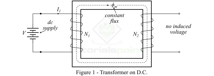
Consider an electrical transformer as shown in Figure-1, and it is connected to a battery (or a source of DC voltage) V. When, we apply this DC voltage V to the primary winding of the transformer, it will draw a constant current (DC) and therefore produces a constant magnetic flux flowing through the magnetic core.
According to the principle of electromagnetic induction, an EMF can induce in a coil or conductor only when it is subjected to a changing magnetic field, i.e.,
$$\mathrm{\mathit{e}\:=\:\mathit{N}\frac{\mathit{d\phi }}{\mathit{dt}}}$$
Consequently, the applied DC voltage to the primary winding does not induce EMF in the primary winding or secondary winding. Hence, this discussion proves that a transformer does not work on DC supply. In fact, connecting a DC supply to the primary winding of a transformer could be dangerous.

The equivalent primary winding circuit of a transformer connected to the DC voltage is shown in Figure-2. In this case, there is no self-induced EMF in the primary winding to oppose the applied voltage V (according to Lenzs law), and the current in the primary winding is given by,
$$\mathrm{\mathit{I_{\mathrm{1}}}\:=\:\frac{\mathit{V}}{\mathit{R_{\mathrm{1}}}}}$$
Where, $\mathit{R_{\mathrm{1}}}$ is the resistance of the primary winding. Due to very small value of R1, the current $\mathit{I_{\mathrm{1}}}$ through the primary winding will be very large. This large current will cause the overheating and burning of the transformer or fuses will blow. Therefore, we must not connect the primary winding of a transformer to the DC supply because it may damage the transformer or may cause an electrical accident.
Losses in a Transformer
The following power losses may occur in a practical transformer −
Iron Loss or Core Loss
Copper Loss or I2R Loss
Stray Loss
Dielectric Loss
In a transformer, these power losses appear in the form of heat and cause two major problems −
Increases the temperature of the transformer.
Reduces the efficiency of the transformer.
Iron Loss or Core Loss
Iron loss occurs in the magnetic core of the transformer due to flow of alternating magnetic flux through it. For this reason, the iron loss is also called core loss. We generally use the symbol ($\mathit{P_{i}}$) to represent the iron loss. The iron loss consists of hysteresis loss ($\mathit{P_{h}}$) and eddy current loss ($\mathit{P_{e}}$). Thus, the iron loss is given by the sum of the hysteresis loss and eddy current loss, i.e.
$$\mathrm{\mathrm{Iron\:loss,}\mathit{P_{i}}\:=\:\mathrm{Hysteresies\:loss(\mathit{P_{h}})}\:+\:\mathrm{Eddy\:current\:loss(\mathit{P_{e}})}}$$
The hysteresis loss and eddy current loss (or iron loss) are determined by performing the open-circuit test on the transformer.
The empirical formulae for the hysteresis loss and eddy current loss are given by,
$$\mathrm{\mathit{P_{h}}\:=\:\mathit{k_{h}f\:B_{m}^{x}}\:\cdot \cdot \cdot (1)}$$
$$\mathrm{\mathit{P_{e}}\:=\:\mathit{ke\:B_{m}^{\mathrm{2}}\:f^{\mathrm{2}}t^{\mathrm{2}}}\:\cdot \cdot \cdot (2)}$$
Where,
The exponent of Bm, i.e. "x" is called the Steinmetzs constant. Depending on the properties of the core material, its value is ranging from 1.5 to 2.5.
kh is a proportionality constant whose value depends upon the volume and quality of the material of core.
ke is a proportionality constant which depend on the volume and resistivity of material of the core.
f is the frequency of the alternating flux in the core.
Bm is the maximum flux density in the core.
t is the thickness of each core lamination.
Therefore, the total iron loss or core loss can also be written as,
$$\mathrm{\mathit{P_{i}}\:=\:\mathit{k_{h}f\:B_{m}^{x}}\:+\:\mathit{ke\:B_{m}^{\mathrm{2}}\:f^{\mathrm{2}}t^{\mathrm{2}}}\:\cdot \cdot \cdot (3)}$$
Since the input voltage to the transformer is approximately equal to the induced voltage in the primary winding, i.e.
$$\mathrm{\mathit{V_{\mathrm{1}}}\:=\:\mathit{E_{\mathrm{1}}}\:=\:4.44\:\mathit{f\phi _{m}N_{\mathrm{1}}}}$$
$$\mathrm{\Rightarrow \mathit{V_{\mathrm{1}}}\:=\:4.44\:\mathit{f\:B_{m}AN_{\mathrm{1}}}}$$
Where, A is the cross-sectional area of the transformer core, N1 is the number of turns in the primary winding and f is the supply frequency.
$$\mathrm{\therefore \mathit{B_{m}}\:=\:\frac{\mathit{V_{\mathrm{1}}}}{4.44\mathit{fAN_{\mathrm{1}}}}\:\cdot \cdot \cdot (4)}$$
Hence, from equations (1) & (4), we get,
$$\mathrm{\mathit{P_{h}}\:=\:\mathit{k_{h}f}\left ( \frac{\mathit{V_{\mathrm{1}}}}{4.44\mathit{fAN_{\mathrm{1}}}} \right )^{x}}$$
$$\mathrm{\Rightarrow \mathit{P_{h}}\:=\:\mathit{k_{h}f}\left ( \frac{\mathrm{1}}{4.44\mathit{AN_{\mathrm{1}}}} \right )^{x}\cdot \left ( \frac{\mathit{V_{\mathrm{1}}}}{\mathit{f}} \right )^{x}}$$
$$\mathrm{\Rightarrow \mathit{P_{h}}\:=\:\mathit{k_{h}}\left ( \frac{\mathrm{1}}{4.44\mathit{AN_{\mathrm{1}}}} \right )^{x}\cdot \mathit{V_{\mathrm{1}}^{x}}\:\mathit{f^{(\mathrm{1}-x)}}\:\cdot \cdot \cdot (5)}$$
Thus, Equation (5) shows that the hysteresis loss depends upon both input voltage and supply frequency.
Again, from equations (2) & (4), we get,
$$\mathrm{\mathit{P_{e}}\:=\:\mathit{k_{e}f^{\mathrm{2}}t^{\mathrm{2}}}\left ( \frac{\mathit{V_{\mathrm{1}}}}{4.44\mathit{fAN_{\mathrm{1}}}} \right )^{\mathrm{2}}}$$
$$\mathrm{\Rightarrow \mathit{P_{e}}\:=\:\mathit{k_{e}\left ( \frac{\mathit{V_{\mathrm{1}}}}{\mathrm{4.44}\mathit{AN_{\mathrm{1}}}} \right )^{\mathrm{2}}\mathit{t^{\mathrm{2}}}\:\cdot \cdot \cdot \mathrm{(6)}}}$$
Hence, from equation (6), we can conclude that the eddy current loss in the transformer is proportional to the square of the input voltage and is independent of the supply frequency.
Therefore, the total core loss can also be written as,
$$\mathrm{\mathit{P_{i}}\:=\:\mathit{k_{h}\left ( \frac{\mathrm{1}}{\mathrm{4.44}\mathit{AN_{\mathrm{1}}}} \right )^{\mathrm{2}}\cdot \mathit{V_{\mathrm{1}}^{\mathit{x}}f^{(\mathrm{1-x})}}\:+\:\mathit{k_{e}}\left ( \frac{V_{\mathrm{1}}}{\mathrm{4.44}\mathit{AN_{\mathrm{1}}}} \right )^{\mathrm{2}}\mathit{t^{\mathrm{2}}}\:\cdot \cdot \cdot \left ( \mathrm{7} \right )}}$$
In practice, transformers are connected to an electric supply of constant frequency and constant voltage, thus, both f and Bm are constant. Therefore, the core or iron loss is practically remains constant at all loads.
We can reduce the hysteresis loss by using steel of high silicon content to construct the core of transformer while the eddy current loss can be minimized by using core of thin laminations instead of solid core. The open-circuit test is performed on a transformer to determine the iron or core loss.
Copper Loss or I2R Loss
Power loss in a transformer that occurs in both the primary and secondary windings due to their Ohmic resistance is called copper loss or I2R loss. We usually represent the copper loss by PC. Therefore, the total copper loss in a transformer is the sum of power loss in the primary winding and power loss in the secondary winding, i.e.,
$$\mathrm{\mathit{P_{c}}\:=\:\mathrm{Copper\:loss\:in\:primary\:+\:Copper\:loss\:in\:secondary}}$$
$$\mathrm{\Rightarrow \mathit{P_{c}}\:=\:\mathit{I_{\mathrm{1}}^{\mathrm{2}}}\mathit{R_{\mathrm{1}}}\:+\:\mathit{I_{\mathrm{2}}^{\mathrm{2}}}\mathit{R_{\mathrm{2}}}\:\cdot \cdot \cdot (8)}$$
Since,
$$\mathrm{\mathit{I_{\mathrm{1}}}\mathit{N_{\mathrm{1}}}\:=\:\mathit{I_{\mathrm{2}}}\mathit{N_{\mathrm{2}}}}$$
$$\mathrm{\Rightarrow \mathit{I_{\mathrm{1}}}\:=\:\left ( \frac{\mathit{N_{\mathrm{2}}}}{\mathit{N_{\mathrm{1}}}} \right )\mathit{I_{\mathrm{2}}}\:\cdot \cdot \cdot (9)}$$
$$\mathrm{\therefore \mathit{P_{c}}\:=\:\left [ \left ( \frac{\mathit{N_{\mathrm{2}}}}{\mathit{N_{\mathrm{1}}}} \right )I_{\mathrm{2}} \right ]^{\mathrm{2}}\:\mathit{R_{\mathrm{1}}}\:+\:\mathit{I_{\mathrm{2}}^{\mathrm{2}}}\mathit{R_{\mathrm{2}}}\:=\:\left [ \left ( \frac{\mathit{N_{\mathrm{2}}}}{\mathit{N_{\mathrm{1}}}} \right )^{\mathrm{2}}\mathit{R_{\mathrm{1}}}\:+\:\mathit{R_{\mathrm{2}}} \right ]\mathit{I_{\mathrm{2}}^{\mathrm{2}}}\:\cdot \cdot \cdot (10)}$$
From Equation (10), it is clear that the copper loss in a transformer varies as the square of the load current. For this reason, the copper loss is also referred as "variable loss" because in practice a transformer is subjected to variable load and hence has variable load current.
We conduct the "short-circuit test" on the transformer to determine the value of its copper loss. In a practical transformer, the copper loss accounts for about 90% of the total power loss in the transformer.
Stray Loss
In practical transformer, a fraction of the total flux follows a path through air and this flux is called leakage flux. This leakage flux produces eddy currents in the conducting or metallic parts like tank of the transformer. These eddy currents cause power loss, which is known as stray loss.
Dielectric Loss
The power loss occurs in insulating materials like oil, solid insulation of the transformer, etc. is known as dielectric loss. The dielectric loss is significant only in transformers working on high voltages.
Although, in practice, the stray loss and dielectric loss are very small, constant and may be neglected.
From the above discussion, we found that a transformer has some losses which are constant and some other are variable. Thus, we may categorize losses in a transformer in two types namely constant losses and variable losses.
Therefore, the total losses in a transformer are the sum of constant losses and variable losses, i.e.,
Total losses in transformer = Constant losses + Variable losses
Efficiency of Transformer
Transformer Efficiency
The ratio of the output power to the input power in a transformer is known as efficiency of transformer. The transformer efficiency is represented by Greek letter Eta ($\eta $).
$$\mathrm{\mathrm{Efficiency,}\eta \:=\:\frac{Output\:Power}{Input\:Power}}$$
From this definition, it appears that we can determined the efficiency of a transformer by directly loading the transformer and measuring the input power and output power. Although, this method of efficiency determination has the following disadvantages −
In practice, the efficiency of a transformer is very high, and a very small error (let say 1%) in input and output wattmeters may give ridiculous results. Consequently, this method may give efficiency more than 100%.
In this method, the transformer is loaded, hence a considerable amount of power is wasted. Therefore, this method becomes uneconomical for large transformers.
It is very difficult to find a load which is capable of absorbing all of the output power.
This method does not provide any information about losses in the transformer.
Thus, due to these limitations, the direct-loading method is rarely used to determine the efficiency of a transformer. In practice, we use open-circuit and short-circuit tests to find out the transformer efficiency.
For a practical transformer, the input power is given by,
$$\mathrm{\mathrm{Input\:power}\:=\:\mathrm{Output\:power\:+\:Losses}}$$
Therefore, the transformer efficiency can also be calculated using the following expression −
$$\mathrm{\eta \:=\:\frac{Output\:power}{Output\:power\:+\:Losses}}$$
$$\mathrm{\Rightarrow \eta \:=\:\frac{VA\times Power\:Factor}{\left ( VA\times Power\:Factor \right )\:+\:Losses}}$$
Where,
$$\mathrm{\mathrm{Output\:power}\:=\:VA\times Power\:factor}$$
And, losses can be determined by transformer tests.
Efficiency from Transformer Tests
When we perform transformer tests, the following results are obtained −
From open-circuit test −
$$\mathrm{\mathrm{Full\:load\:iron\:loss}\:=\:\mathit{P_{i}}}$$
From short-circuit test −
$$\mathrm{\mathrm{Full\:load\:copper\:loss}\:=\:\mathit{P_{c}}}$$
Therefore, the total losses at full load in a transformer are
$$\mathrm{\mathrm{Total\:FL\:losses}\:=\:\mathit{P_{i}+\:P_{c}}}$$
Now, we are able to determine the full-load efficiency of the transformer at any power factor without actual loading the transformer.
$$\mathrm{\mathit{n_{FL}}\:=\:\frac{(VA)_{\mathit{FL}}\times Power\:factor}{[(VA)_{\mathit{FL}}\times Power\:factor]+\:\mathit{P_{i}}+\mathit{P_{c}}}}$$
Also, the transformer efficiency at any load equal to x full load. Where, x is the fraction of loading. In this case, the total losses corresponding to the given load are,
$$\mathrm{(Total\:losses)_{x}\:=\:\mathit{P_{i}+\:x^{\mathrm{2}}\mathit{P_{c}}}}$$
It is because, the iron loss ($\mathit{P_{i}}$) is the constant loss and hence remains the same at all loads, while the copper loss is proportional to the square of the load current.
$$\mathrm{\therefore\eta _{x}\:=\: \frac{\mathit{x}\times (VA)_{\mathit{FL}}\times Power\:factor}{[\mathit{x}\times (VA)_{\mathit{FL}}\times Power\:factor]+\:\mathit{P_{i}}+\:x^{\mathrm{2}}\mathit{P_{c}}}}$$
Condition for Maximum Efficiency
For a given transformer, we have,
$$\mathrm{\mathrm{Output\:power}\:=\:\mathit{V_{\mathrm{2}}I_{\mathrm{2}}cos\phi _{\mathrm{2}}}}$$
Let the transformer referred to secondary side, then Ro2 is the total resistance of the transformer. The total copper loss is given by,
$$\mathrm{\mathit{P_{c}}\:=\:\mathit{I_{\mathrm{2}}^{\mathrm{2}}\mathit{R_{o\mathrm{2}}}}}$$
Therefore, the transformer efficiency is given by,
$$\mathrm{\eta \:=\:\frac{\mathit{V_{\mathrm{2}}}I_{\mathrm{2}}cos\phi _{\mathrm{2}}}{\mathit{V_{\mathrm{2}}I_{\mathrm{2}}cos\phi _{\mathrm{2}}}+\mathit{P_{i}}+\mathit{I_{\mathrm{2}}^{\mathrm{2}}}R_{o\mathrm{2}}}}$$
On rearranging the expression, we get,
$$\mathrm{\eta \:=\:\frac{\mathit{V_{\mathrm{2}}}cos\phi _{\mathrm{2}}}{\mathit{V_{\mathrm{2}}cos\phi _{\mathrm{2}}}+\left ( \mathit{\frac{P_{i}}{I_{\mathrm{2}}}} \right )+\mathit{I_{\mathrm{2}}}R_{o\mathrm{2}}}\:=\:\mathit{\frac{V_{\mathrm{2}}cos\phi _{\mathrm{2}}}{D}}\:\cdot \cdot \cdot (1)}$$
In practice, the secondary voltage V2 is approximately constant. Hence, for a load of given power factor, the transformer efficiency depends upon the load current (I2). From the equation (1), we can see that the numerator is constant and for the efficiency to be maximum, the denominator (D) should be minimum, i.e.
$$\mathrm{\mathit{\frac{d(D)}{dI_{\mathrm{2}}}}\:=\:0}$$
$$\mathrm{\Rightarrow\mathit{\frac{d}{dI_{\mathrm{2}}}}\left [ \mathit{V_{\mathrm{2}}cos\phi _{\mathrm{2}}}+\left ( \mathit{\frac{P_{i}}{I_{\mathrm{2}}}}\right )+\mathit{I_{\mathrm{2}} R_{0\mathrm{2}}} \right ]\:=\:0}$$
$$\mathrm{\Rightarrow 0-\left ( \mathit{\frac{P_{i}}{I_{\mathrm{2}}}} \right )+\mathit{R_{o\mathrm{2}}}\:=\:0}$$
$$\mathrm{\Rightarrow \mathit{P_{i}}\:=\:\mathit{I_{\mathrm{2}}^{\mathrm{2}}R_{o\mathrm{2}}}}$$
$$\mathrm{\Rightarrow \mathrm{Iron\:loss}\:=\:Copper\:loss}$$
Therefore, the transformer efficiency for a given power factor will be maximum when the constant iron loss is equal to the variable copper loss.
The maximum efficiency at any load is given by,
$$\mathrm{\mathit{\eta _{max}}\:=\:\frac{\mathit{x\times (VA)_{\mathit{FL}}\times \mathrm{Power\:factor}}}{[\mathit{x\times (VA)_{\mathit{FL}}}\times Power\:fctor]+\:2\mathit{P_{i}}}}$$
Also, the load current (I2) corresponding to the maximum efficiency of transformer is,
$$\mathrm{\mathit{I_{\mathrm{2}}}\:=\:\sqrt{\frac{\mathit{P_{i}}}{R_{o2}}}}$$
Numerical Example
In a 100 kVA transformer, the iron loss is 450 W and full-load copper loss is 900 W. Find the transformer efficiency at full load and the maximum efficiency of the transformer, where the load power factor is 0.8 lagging.
Solution
Given data,
Full load VA = 100 kVA = 100 1000 VA
Iron loss,Pi = 450 W
Copper loss,Pc = 900 W
cos$\mathit{\phi _{\mathrm{2}}}$ = 0.8
Transformer efficiency at full-load −
$$\mathrm{\mathrm{Total\:losses}\:=\:450\:+\:900\:=\:1350\:W}$$
$$\mathrm{\mathit{\eta _{\mathit{FL}}}\:=\:\frac{(VA)_{\mathit{FL}}\times Power\:factor}{[(VA)_{\mathit{FL}}\times Power\:factor]+\:Total\:losses}}$$
$$\mathrm{\Rightarrow \mathit{\eta _{\mathit{FL}}}\:=\:\frac{100\times 1000\times 0.8}{(100\times 1000\times 0.8)+1350}\:=\:\frac{80000}{81350}\:=\:0.9834}$$
$$\mathrm{\therefore \eta _{\mathit{FL}}\:=\:0.9834\times 100\%\:=\:98.34\%}$$
Maximum efficiency of the transformer −
For maximum efficiency,
$$\mathrm{\mathrm{Iron\:loss}\:=\:Copper\:Loss}$$
$$\mathrm{\therefore \eta _{\mathit{max}}\:=\:\frac{(VA)_{\mathit{FL}}\times Power\:factor}{[(VA)_{\mathit{FL}}\times Power\:factor]+2\mathit{P_{i}}}}$$
$$\mathrm{\Rightarrow \eta _{\mathit{max}}\:=\:\frac{100\times 1000\times 0.8}{(100\times 1000\times 0.8)+(2\times 450)}\:=\:0.9888}$$
$$\mathrm{\therefore \eta _{\mathit{max}}\:=\:0.9888\times 100\%\:=\:98.88\%}$$
Three-Phase Transformer
In practice, electrical power is generated, transmitted and distributed by using three-phase system. Therefore, we require a three-phase transformer to step-up or step-down the voltage at various stages of a power system network.
We can construct a three-phase transformer in one of the following two ways −
We can connect three separate single-phase transformers for 3-phase operation. This arrangement is known as a three-phase bank of transformers.
We can construct a single three-phase transformer which consists of a magnetic core and having windings for all the three phases. This whole assembly is combined in a single structure.
The windings of a three-phase transformer may be connected in the following ways −
Star-Star Connection − In this case, both primary and secondary windings are connected in star connection.
Delta-Delta Connection − In this case, both primary and secondary windings are connected in delta connection.
Delta-Star Connection − In this case, the primary winding is connected in delta, while the secondary winding is connected in star.
Star-Delta Connection − In this case, the primary winding is connected in star while the secondary winding is connected in delta.
Construction of Three Phase Transformer
A three phase transformer can be constructed in two ways namely core-type construction and shell-type construction.
Core Type Construction
In the core type construction of 3-phase transformer, the magnetic core has three vertical limbs and two horizontal sections as shown in Figure-1. Here, one pair of primary and secondary windings is placed on each limb. The low voltage (lv) winding is placed next to the core while the high-voltage (hv) winding is wound around the lv winding.
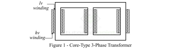
Shell Type Construction
A shell type three-phase transformer can be constructed by stacking three single-phase shell-type transformers together as shown in Figure-2. In this case, both primary and secondary windings are placed on the central limb and the two outer limbs serve the path for flux. The behavior of a shell-type three-phase transformer is almost similar to that of a bank of three single-phase transformers.
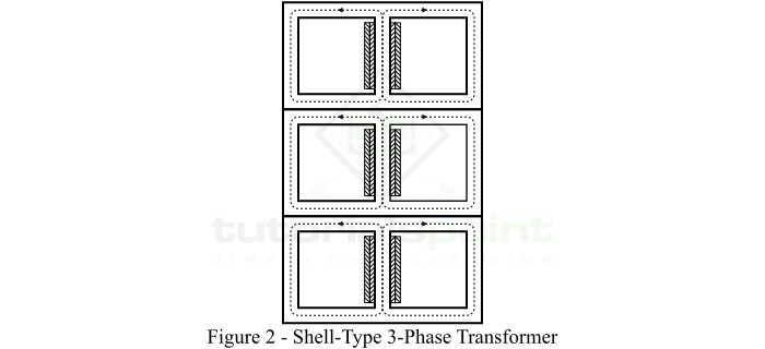
Advantages of a Bank of Three Single Phase Transformers
The following are the major advantages that a bank of three single-phase transformers have over a three-phase unit transformer −
When one 1-phase transformer of a bank of transformers is damaged and isolated from the service, the remaining two transformers may be used to supply power in open-delta connection.
In the bank of transformers, we can provide a single-phase transformer with higher kVA rating than the others to supply an imbalance load.
For a bank of three single-phase transformers, the standby requirement is lesser.
It is more convenient to transport a 1-phase transformer than a 3-phase transformer.
Advantages of a Three Phase Unit Transformer
For the same kVA rating, a three-phase unit transformer has the following advantages over a bank of three single-phase transformers −
A three-phase unit transformer is smaller in size, light in weight and cheaper.
It is more efficient than bank of transformers.
Its installation is simple.
Depending upon the requirements, we use both bank of transformers and a three-phase unit transformer. However, it is a common practice to use a three-phase unit transformer.
Types of Transformers
Depending on the number of turns in primary and secondary windings, the transformers may be classified into the following three types −
Step-up transformer
Step-down transformer
One-to-one transformer
Depending on the application, we may classify the transformers in the following three main types
Power transformers
Distribution transformers
Instrument transformers
Step-Up Transformer
A transformer in which the number of turns in the secondary winding are greater than the number of turns in the primary winding, as a result its output voltage is greater than the input voltage is known as a step-up transformer. In power systems, the step-up transformer is used to increase the low voltages to a higher value for transmission purposes.
Step-Down Transformer
A transformer in which the number of turns in the secondary winding are less than that in the primary winding as a result the output voltage is less than the input voltage is known as a step-down transformer. In power systems, the step-down transformers are used to decrease the high-voltages to a lower value for distribution and utilization purposes.
One-to-One (1:1) Transformer
A transformer in which the number of turns in both primary winding and secondary winding are same so that it produces an output voltage equal to the input voltage is known as a one-to-one transformer. It is also known as isolation transformer. It finds application in such areas where two electrical circuits are required to be isolated electrically, but coupled magnetically for power transfer.
Power Transformers
A transformer with high volt-ampere (VA) rating, commonly of the order of Mega or Giga, is referred as a power transformer. The power transformers are designed to operate with an almost constant load which is equal to their rating. These transformers are used in generating stations, receiving stations and substations at ends of the power transmission lines for stepping-up or stepping-down the voltage.
In practice, power transformers are put into operation during load periods while they are disconnected during light load periods. These transformers are designed to have maximum efficiency at or near full-load. However, power transformers are so designed that they have considerably high leakage reactance. Thus, for power transformers the current limiting effect of high leakage reactance is more important than the voltage regulation.
Distribution Transformers
The transformer which is used to reduce the high voltage to a low value for distribution purpose is known as a distribution transformer. Distribution transformers are designed to operate with variable load which is considerably less than their rating. Therefore, these transformers are designed to have maximum efficiency at the load between and of the full-load. Distribution transformers are kept in operation all the 24 hours of a day whether they are carrying any load or not. Distribution transformers have a good voltage regulation, and are designed to have a small value of leakage reactance.
Instrument Transformers
It is very difficult to measure high alternating currents and voltages with simple measuring devices. Thus, to make the measurement of high alternating currents and voltages simple, we use specially designed transformers, called instrument transformers. By employing instrument transformers, we can measure high alternating quantities with low-range AC measurement devices.
Depending on the type of quantity transformed, instrument transformers are of the following two types −
Current Transformer (C.T.)
Potential Transformer (P.T.)
Current Transformer
A current transformer is a type of instrument transformer which is used to decrease the high alternating current of power line to a measurable low value. Basically, a current transformer is a voltage step-up and current step-down transformer. It has a primary winding of a few turns of thick wire, and a secondary winding having more turns of fine wire. The primary winding of CT is connected in series with the line whose current is to be measured, and the secondary winding is connected across a low-range AC ammeter to measure and indicate the current.
Potential Transformer
A potential transformer is a voltage step-down transformer which is used to reduce the high line voltages to a measurable value. The primary winding of a PT has many turns while the secondary winding has few turns. The primary winding is connected across the power line whose voltage is to be measured and the secondary winding is connected across a low-range AC voltmeter to indicate the measured voltage value.
Construction of DC Machines
An electromechanical device which can convert direct current (dc) electricity into mechanical energy or mechanical energy into direct current (dc) electricity is known as a DC machine.
If the DC machine converts DC electrical energy into mechanical energy, it is known as DC motor. If the machine converts mechanical energy into DC electrical energy, then it is known as a DC generator. Both DC motor and DC generator have the similar construction.
A typical DC machine consists of the following major parts −
Yoke or Frame
Armature
Field System
Commutator
Brushes
Bearings
The schematic diagram of a DC machine is shown below −
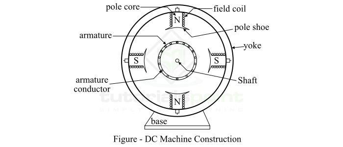
Let us now discuss each of these components in greater detail.
Yoke or Frame
The yoke is the outer frame of the DC machine. It is made up of such materials that have high permeability and high mechanical strength. In practice, the yoke of DC machine is made up of cast steel.
The yoke or frame of the DC machine serves the following main purposes −
It protects the internal machine parts like armature, windings, field poles, etc. against mechanical damages.
The yoke houses the magnetic field system.
It provides a low reluctance path to the working magnetic flux.
It supports the rotor or armature through bearings.
Armature
In DC machines (motor or generator), armature is a system of conductors or coils that can rotate freely on the supporting bearings. The working torque and EMF are developed in coils of the armature. The armature consists of two main parts namely, armature core and armature winding.
The armature core is a solid cylindrical structure, made up of high permeability thin silicon steel laminations. On the outer periphery of the core slots are cut to carry the armature winding.
The armature winding is made up of copper wires. The armature winding of DC machine is generally former wound. Depending upon the end connections of the armature conductors, the armature winding may be of two types namely lap winding and wave winding. The type of winding decides the voltage and current rating of the machine. In case of the lap winding, the number of parallel paths (A) for current to flow are equal to the number of poles (P) in the machine. On the other hand, for wave winding, the number of parallel paths (A) are equal to 2.
Field System
Field system is the part of a DC machine which produces the working magnetic flux in the machine. It is basically a system of electromagnets which is excited by a DC supply. In case of DC machine, the field system is a stationary part of the machine and it is bolted to the yoke or frame of the machine. There are three main parts of a field system in dc machines namely pole core, pole shoes, and field coils.
The pole core is made up of thin steel laminations. One end of the pole core is bolted to the frame and other end has pole shoe. The pole core carries the field winding.
The pole shoe is a projected part of the pole core and has a large area of cross-section. Pole shoes help in spreading the magnetic flux uniformly in the air gap, and offers low reluctance path to the magnetic flux. Also, it supports the field winding.
The field coil or winding is made up of copper wire. The field winding is former wound and inserted around the pole core. When field windings are excited by DC supply, they become electromagnets and produce magnetic flux in the machine.
Commutator
The commutator is one of the important parts of the DC machine. It is basically mechanical rectifier. It is a cylindrical shaped device and is made up of copper. The outer periphery of the commutator has V-shaped slots to carry commutator segments. Where, the commutator segments are copper bars inserted in the slots. These segments are insulated from each other by mica. The commutator is mounted on the shaft of the DC machine on one side of the armature. The armature conductors are connected to the commutator segments with the help of copper lugs.
The commutator performs the following two major functions −
In a DC generator, it collects the current from the armature conductor. In a DC motor, it supplies the current to the armature conductors.
It converts the alternating current of the armature into unidirectional current in the external circuit with the help of brushes, and vice-versa.
Brushes
Brushes are used to make an electrical connection with the rotating commutator. These collect (or supply) current from (or to) the moving commutator. Brushes are usually made up of carbon. They are housed in brush holders and are in contact with the commutator surface with the help of spring pressure.
Bearings
Bearings are used in the DC machine to reduce the frictional losses. Thus, the main function of bearings in the DC machine is to support the machine shaft with minimum friction. In DC machines, ball bearings or roller bearings are commonly used.
Types of DC Machines
A DC machine is a device which converts electrical energy in the form of direct current into mechanical energy or mechanical energy into electrical energy in the form of direct current. Therefore, a DC machine is basically an electromechanical energy conversion device.
Based on the energy conversion, DC machines can be classified into the following two types −
DC Motor
DC Generator
The basic construction of both DC motor and DC generator is almost similar. However, the fundamental principles involved in the operation of DC motor and DC generator are different.
Every DC machine essentially consists of a system of conductors and system of magnets or electromagnets. The system of conductor is called armature, and in case of DC machines it is mounted on a movable shaft. The system of magnets or electromagnets is known as the field system, and it produces the required working magnetic flux.
DC Motor
The block diagram of a DC motor is shown in Figure-1.
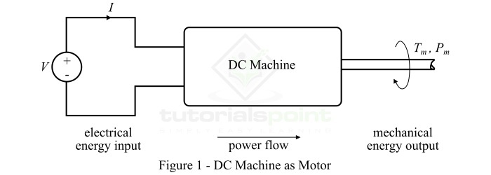
When the DC machine is designed to convert DC electrical energy into rotational mechanical energy, it is called a DC motor. Therefore, in case of a DC motor, the electrical energy is supplied to the machine through input terminals and mechanical energy output is taken from the shaft in the form of rotation of the shaft.
DC Generator
The block diagram of a DC generator is shown in Figure-2.
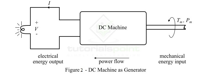
A DC machine which can convert mechanical energy input into electrical energy output is known as a DC generator. Thus, in a DC generator, the mechanical energy from a source like engine, turbine, etc. is supplied to the DC machine in the form of rotational energy of the shaft and the DC electrical energy is received as output from the armature terminals.
Working Principle of DC Generator
The working principle of DC generator is based on the Faradays law of electromagnetic induction. According to this law, when the magnetic flux liked to a conductor or coil changes an EMF is induced in the conductor or coil. The magnitude of this induced EMF is given by,
$$\mathrm{\mathit{e}\:=\:\mathit{N}\frac{\mathit{d\phi }}{\mathit{dt}}\:\cdot \cdot \cdot (1)}$$
Where, $\phi$ is the flux linkage of the coil and N is the number of turns in the coil.
In case of a DC generator, the magnetic flux ($\phi$) remains stationary and the coil rotates. The EMF induced where the coil is rotating and flux is stationary, is known as dynamically induced EMF.
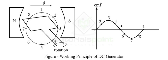
In order to understand the working principle of a DC generator, we consider a single loop DC generator (i.e. N = 1) as shown in above figure. Here, the coil is rotated by some prime mover (a source of mechanical energy), and there is a change in the magnetic flux linkage to the coil.
Let $\phi$ be the average magnetic flux produced by each magnetic pole of the machine, then the average induced EMF in the generator is given by,
$$\mathrm{\mathit{E_{av}}\:=\:\frac{\mathit{d\phi }}{\mathit{dt}}\:=\:\mathrm{Flux\: cut\: per\:sec\:by\: the \:coil}}$$
$$\mathrm{\Rightarrow \mathit{E_{av}}\:=\:\mathrm{Flux\: cut\: in \:one \:rotation\:\times \:No.\:of\: rotations\: per\: sec}}$$
$$\mathrm{\Rightarrow \mathit{E_{av}}\:=\:\mathrm{\left ( Flux\:per\:pole\times No.\:of\:poles \right )}\:\times \:\mathrm{No.\:of \:rotations \:per\: sec}}$$
$$\mathrm{\therefore \mathit{E_{av}}\:=\:\mathit{\phi \:\times P\:\times \:n}\:\cdot \cdot \cdot (2)}$$
Where, P is the total number of poles in the generator and n is the speed of the coil in rotation per second. The expression in the Equation-(2) gives the average induced EMF in a single loop DC generator.
The following points explain the working principle of a DC generator −
Position 1 − The induced EMF is zero because, the movement of coil sides is parallel to the magnetic flux.
Position 2 − The coil sides are moving at an angle to the magnetic flux, and hence a small EMF is generated in the loop.
Position 3 − The coil sides are moving at right angle to the magnetic flux, therefore the induced EMF is maximum.
Position 4 − The coil sides are cutting the magnetic flux at an angle, thus a reduced EMF is induced in the coil sides.
Position 5 − No flux linkage with the coil side and the coil sides are moving parallel to the magnetic flux. Therefore, no EMF is induced in the coil.
Position 6 − The coil sides move under a pole of opposite polarity and hence the polarity of induced EMF is reversed. The maximum EMF will induce in this direction at position 7 and zero when it is at position 1. This cycle repeats with rotation of the coil.
In this way, EMF is induced in a DC generator. Though, this induced EMF is alternating in nature, which is then converted in the unidirectional EMF by using a device called commutator.
The direction of induced EMF in the armature conductor of the DC generator is determined by the Fleming right hand rule (FRHR) which we discussed in the module-1 (basic concepts) of this tutorial.
EMF Equation of DC Generator
The expression which gives the magnitude of EMF generated in a DC generator is called EMF equation of DC generator. We shall now drive the expression for the EMF induced in a DC generator.
Let,
$\phi $ = flux per pole
P = number of poles in the generator
Z = no.of armature coductors
A = no.of parallel paths
N = speed of armature in RPM
E = EMF generated
Thus, the magnetic flux (in weber) cut by a conductor in one revolution of the armature is given by,
$$\mathrm{\mathit{d\phi \:=\:P\times \phi }}$$
If N is the number of revolution per minute, then the time (in seconds) taken complete one revolution is,
$$\mathrm{\mathit{dt \:=\frac{60}{N}}}$$
According to Faradays law of electromagnetic induction, the EMF induced per conductor is given by,
$$\mathrm{\mathrm{EMF/conductor}\:=\:\mathit{\frac{d\phi }{dt}}\:=\:\frac{\mathit{P\phi }}{\mathrm{\left ( {60/\mathit{N}} \right )}}\:=\:\frac{\mathit{P\phi N}}{\mathrm{60}}}$$
The total EMF generated in the generator is equal to the EMF per parallel path, which is the product of EMF per conductor and the number of conductors in series per parallel path, i.e.,
$$\mathrm{\mathit{E}\:=\:\left ( EMF/Conductor \right )\times \left ( No.\:of\:conductors/parallel\:path \right )}$$
$$\mathrm{\Rightarrow \mathit{E}\:=\:\frac{\mathit{P\phi N}}{60}\times \frac{\mathit{Z}}{\mathit{A}}}$$
$$\mathrm{\therefore \mathit{E}\:=\:\frac{\mathit{NP\phi N}}{60\mathit{A}}\:\cdot \cdot \cdot \left ( 1 \right )}$$
Equation (1) is called the EMF equation of DC generator.
For wave winding,
$$\mathrm{\mathrm{Number\:of\:parllel\:paths,}\mathit{A}\:=\:2}$$
$$\mathrm{\therefore \mathit{E}\:=\:\frac{\mathit{NP\phi Z}}{\mathrm{120}}}$$
For lap winding,
$$\mathrm{\mathrm{Number\:of\:parllel\:paths,}\mathit{A}\:=\:\mathit{P}}$$
$$\mathrm{\therefore \mathit{E}\:=\:\frac{\mathit{N\phi Z}}{\mathrm{60}}}$$
For a given DC generator, Z, P and A are constant so that the generated EMF (E) is directly proportional to flux per pole ($\phi$) and speed of armature rotation (N).
Numerical Example
A 6-pole dc generator has 600 armature conductors and a useful flux of 0.06 Wb. What will be the EMF generated, if it is wave connected and lap connected and runs at 1000 RPM?
Solution:
Given data,
No.of poles,P = 6
No.of armature conductors,Z = 600
Flux per pole,$\phi$ = 0.06 Wb
Speed of armature,N = 1000 RPM
For wave-connected generator,
$$\mathrm{\mathit{E}\:=\:\frac{\mathit{NP\phi Z}}{\mathrm{120}}}$$
$$\mathrm{\Rightarrow \mathit{E}\:=\:\frac{1000\times6\times 0.06\times 600}{120}}$$
$$\mathrm{\therefore \mathit{E}\:=\:1800\:V}$$
For lap-connected generator,
$$\mathrm{\mathit{E}\:=\:\frac{\mathit{N\phi Z}}{\mathrm{60}}}$$
$$\mathrm{\Rightarrow \mathit{E}\:=\:\frac{1000\times 0.06\times 600}{60}}$$
$$\mathrm{\therefore \mathit{E}\:=\:600\:V}$$
Types of DC Generators
In practical DC generators, the magnetic field is produced by electromagnets rather than permanent magnets. The DC generators are then classified based on the connection of field winding in the generator circuit. On this basis, DC generators are classified into the following two types −
Separately Excited DC Generators
Self-Excited DC Generators
Separately Excited DC Generator
A DC generator whose magnetic field winding is excited from an independent source of DC electric supply like battery is called a separately excited DC generator. Figure-1 shows the connection diagram of a separately excited DC generator.
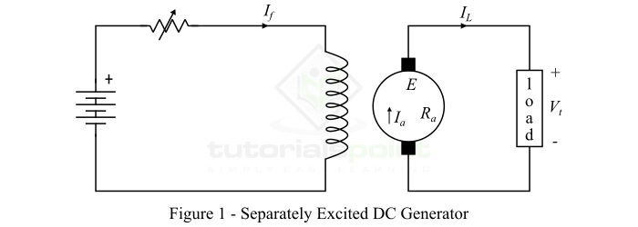
The voltage generated by a separately excited DC generator depends upon the speed of the armature rotation and the field current (i.e. flux in the machine). The greater the speed of armature and field current, greater is the induced EMF in the generator. However, the separately excited DC generators are rarely used in practical applications because these require an external source of DC power for field excitation.
Self-Excited DC Generators
The type of DC generator whose magnetic field winding is excited from the output of the generator itself is known as a self-excited DC generator. Depending upon the manner in which the field winding is connected to the armature, self-excited DC generators are classified into the following three types −
Series DC generator
Shunt DC generator
Compound DC generator
Series DC Generator
A dc generator whose field winding is connected in series with the armature so that whole armature current flows through the field winding as well as the load is called a series DC generator. Figure-2 shows the connection diagram of a series DC generator.
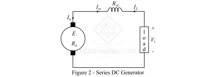
In case of series dc generator, the field winding carries the whole load current, thus it is made up of thick wire with a few turns, so it possesses minimum resistance. The series DC generator is used in special applications like boosters, etc.
The following are some important expressions for the series DC generator −
$$\mathrm{\mathrm{Armature\:current},\mathit{I_{a}}\:=\:\mathit{I_{se}}\:=\:\mathit{I_{L}}}$$
Where,$\mathit{I_{se}}$ is the series field current and $\mathit{I_{L}}$ is the load current.
$$\mathrm{\mathrm{Terminal\:voltage},\mathit{V_{t}}\:=\:\mathit{E-I_{a}\left ( \mathit{R_{a}+R_{se}} \right )}}$$
Where, E is the generated EMF, $\mathit{R_{a}}$ is the armature circuit resistance,$\mathit{R_{se}}$ is the series field resistance.
Shunt DC Generator
A DC generator whose field winding is connected in parallel with the armature winding so that terminal voltage of the generator is applied across it, is known as a shunt DC generator. Figure-3 shows the connection diagram of a shunt DC generator.
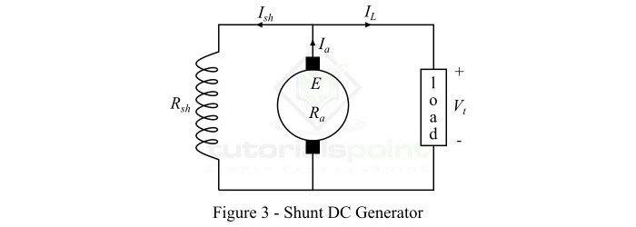
In a shunt DC generator, the shunt field winding has a large number of turns of thin wire so it has high resistance, and therefore only a part of armature current flows through it and the rest flows through the load.
The following are important expressions of a shunt DC generator −
$$\mathrm{\mathrm{Armature\:current,}\mathit{I_{a}}\:=\:\mathit{I_{L}+I_{sh}}}$$
$$\mathrm{\mathrm{Shunt\:field\:current,}\mathit{I_{sh}}\:=\:\frac{\mathit{V_{t}}}{\mathit{R_{sh}}}}$$
$$\mathrm{\mathrm{Terminal\:voltage},\mathit{V_{t}}\:=\:\mathit{E-I_{a}R_{a}}}$$
Compound DC Generator
A compound dc generator is one which has two sets of field windings on each magnetic pole one is in series and the other is in parallel with the armature winding. The compound dc generators may further be divided into the following two types −
Short-shunt compound DC generator
Long-shunt compound DC generator
A short-shunt compound DC generator is one in which only shunt field winding is in parallel with the armature winding as shown in Figure-4.
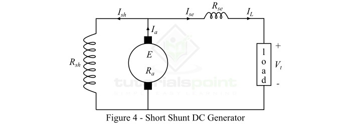
A long-shunt compound DC generator is one in which shunt field winding is in parallel with both series field winding and armature winding as shown in Figure-5.
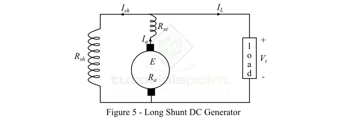
The following are important expressions for compound DC generators −
For short-shunt generator,
$$\mathrm{\mathrm{Armature\:current,}\mathit{I_{a}}\:=\:\mathit{I_{L}+I_{sh}}}$$
$$\mathrm{\mathrm{Series\:field\:current,}\mathit{I_{se}}\:=\:\mathit{I_{L}}}$$
$$\mathrm{\mathrm{Shunt\:field\:current,}\mathit{I_{sh}}\:=\:\frac{\mathit{V_{t}}+\mathit{I_{se}R_{se}}}{R_{sh}}}$$
$$\mathrm{\mathrm{Terminal\:voltage},\mathit{V_{t}}\:=\:\mathit{E-I_{a}R_{a}-I_{se}R_{se}}}$$
For long-shunt generator,
$$\mathrm{\mathrm{Armature\:current,}\mathit{I_{a}}\:=\:\mathit{I_{L}+I_{sh}}}$$
$$\mathrm{\mathrm{Series\:field\:current,}\mathit{I_{se}}\:=\:\mathit{I_{a}}}$$
$$\mathrm{\mathrm{Shunt\:field\:current,}\mathit{I_{sh}}\:=\:\frac{\mathit{V_{t}}}{\mathit{R_{sh}}}}$$
$$\mathrm{\mathrm{Terminal\:voltage},\mathit{V_{t}}\:=\:\mathit{E-I_{a}}\left ( \mathit{R_{a}+R_{se}} \right )}$$
Working Principle of DC Motor
The working principle of DC generator is based on the Faradays law of electromagnetic induction. According to this law, when the magnetic flux liked to a conductor or coil changes an EMF is induced in the conductor or coil. The magnitude of this induced EMF is given by,
$$\mathrm{\mathit{e}\:=\:\mathit{N}\frac{\mathit{d\phi }}{\mathit{dt}}\:\cdot \cdot \cdot (1)}$$
Where, $\phi$ is the flux linkage of the coil and N is the number of turns in the coil.
In case of a DC generator, the magnetic flux ($\phi$) remains stationary and the coil rotates. The EMF induced where the coil is rotating and flux is stationary, is known as dynamically induced EMF.
In order to understand the working principle of a DC generator, we consider a single loop DC generator (i.e. N = 1) as shown in above figure. Here, the coil is rotated by some prime mover (a source of mechanical energy), and there is a change in the magnetic flux linkage to the coil.
Let $\phi$ be the average magnetic flux produced by each magnetic pole of the machine, then the average induced EMF in the generator is given by,
$$\mathrm{\mathit{E_{av}}\:=\:\frac{\mathit{d\phi }}{\mathit{dt}}\:=\:\mathrm{Flux\: cut\: per\:sec\:by\: the \:coil}}$$
$$\mathrm{\Rightarrow \mathit{E_{av}}\:=\:\mathrm{Flux\: cut\: in \:one \:rotation\:\times \:No.\:of\: rotations\: per\: sec}}$$
$$\mathrm{\Rightarrow \mathit{E_{av}}\:=\:\mathrm{\left ( Flux\:per\:pole\times No.\:of\:poles \right )}\:\times \:\mathrm{No.\:of \:rotations \:per\: sec}}$$
$$\mathrm{\therefore \mathit{E_{av}}\:=\:\mathit{\phi \:\times P\:\times \:n}\:\cdot \cdot \cdot (2)}$$
Where, P is the total number of poles in the generator and n is the speed of the coil in rotation per second. The expression in the Equation-(2) gives the average induced EMF in a single loop DC generator.
The following points explain the working principle of a DC generator −
Position 1 − The induced EMF is zero because, the movement of coil sides is parallel to the magnetic flux.
Position 2 − The coil sides are moving at an angle to the magnetic flux, and hence a small EMF is generated in the loop.
Position 3 − The coil sides are moving at right angle to the magnetic flux, therefore the induced EMF is maximum.
Position 4 − The coil sides are cutting the magnetic flux at an angle, thus a reduced EMF is induced in the coil sides.
Position 5 − No flux linkage with the coil side and the coil sides are moving parallel to the magnetic flux. Therefore, no EMF is induced in the coil.
Position 6 − The coil sides move under a pole of opposite polarity and hence the polarity of induced EMF is reversed. The maximum EMF will induce in this direction at position 7 and zero when it is at position 1. This cycle repeats with rotation of the coil.
In this way, EMF is induced in a DC generator. Though, this induced EMF is alternating in nature, which is then converted in the unidirectional EMF by using a device called commutator.
The direction of induced EMF in the armature conductor of the DC generator is determined by the Fleming right hand rule (FRHR) which we discussed in the module-1 (basic concepts) of this tutorial.
Back EMF in DC Motor
In a DC motor, when the armature rotates under the influence of the driving torque, the armature conductors move through the magnetic field, and therefore an EMF is induced in them by the generator action. This induced EMF in the armature conductors acts in opposite direction to the applied voltage $\mathit{V_{s}}$ and is known as the back EMF or counter EMF.
The magnitude of the back EMF is given by,
$$\mathrm{\mathit{E_{b}}\:=\:\frac{\mathit{NP\phi Z}}{\mathrm{60}\mathit{A}}\:\cdot \cdot \cdot (1)}$$
The back EMF $\mathit{E_{b}}$ is always less than the applied voltage $\mathit{V_{s}}$. However, this difference is small when the DC motor is running under normal conditions.
In DC motors, the back EMF $\mathit{E_{b}}$ induced in the armature opposes the applied voltage, thus the applied voltage has to overcome this EMF $\mathit{E_{b}}$ to force a current $\mathit{I_{a}}$ in the armature circuit for motor action. The required power to overcome this opposition is given by,
$$\mathrm{\mathit{P_{m}}\:=\:\mathit{E_{b}I_{a}}\:\cdot \cdot \cdot (2)}$$
The power $\mathit{P_{m}}$ is one which actually converted into mechanical power. For this reason, the power $\mathit{P_{m}}$ is also called as electrical equivalent of mechanical power developed.
Consider a shunt DC motor whose electrical equivalent circuit is shown in Figure-1.
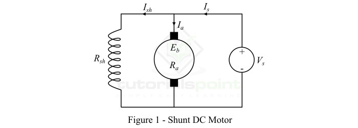
When a DC voltage $\mathit{V_{s}}$ is applied across terminals of the motor, the field electromagnets are excited and armature conductors are supplied with current. Hence, a driving torque acts on the armature which begins to rotate. When the armature rotates, a back EMF is induced in the armature conductors that opposes the applied voltage $\mathit{V_{s}}$. This applied voltage has to force a current through the armature conductors against the back EMF.
The voltage equation of the dc motor can be expressed as,
$$\mathrm{\mathit{V_{s}\:=\:E_{b}+I_{a}R_{a}}\:\cdot \cdot \cdot (3)}$$
Where,$\mathit{R_{a}}$ is the resistance of the armature circuit.
Then, the armature current of the DC motor is given by,
$$\mathrm{\mathit{I_{a}}\:=\:\frac{\mathit{V_{s}-E_{b}}}{\mathit{R_{a}}}\:\cdot \cdot \cdot (4)}$$
Since the applied voltage $\mathit{V_{s}}$ and armature resistance $\mathit{R_{a}}$ are usually fixed for a given motor, then the value of $\mathit{E_{b}}$ will determine the current drawn by the DC motor. If the speed of the DC motor is high, then the value of back EMF is large and hence the motor will draw less armature current and vice-versa.
Significance of Back EMF in DC Motor
The back EMF in a DC motor makes it a self-regulating machine, which means it makes the motor to draw a sufficient amount of armature current to develop the torque required by the mechanical load.
Now, from Equation-4, we may explain the importance of back EMF in the DC motor as −
Case 1 − Motor running on no load
In this case, the dc motor requires a small torque to overcome the frictional and windage losses. Thus, the armature current $\mathit{I_{a}}$ drawn by the motor is small and the back EMF is nearly equal to the supply voltage.
Case 2 − Motor load is changed suddenly
In this case, when load is suddenly attached to the motor shaft, the armature slows down. Consequently, the speed at which the armature conductors move through the magnetic field is decreased and hence the back EMF decreases. This decreased back EMF allows a larger current to pass through the armature conductors, and larger armature current means high driving torque. Hence, it is clear that the driving torque increases as the motor speed decreases. The reduction in motor speed stops when the armature current is sufficient to produce the increased torque required by the mechanical load.
Consider another situation, where the load on the motor is decreased. In this case, the driving torque is momentarily more than the requirement so that the armature is accelerated. The increase in the armature speed increases the back EMF, and causes the armature current to decrease. Once the armature current is just sufficient to produce the reduced driving torque required by the load, the motor will stop accelerating.
This discussion clears that the back EMF in a dc motor automatically regulates the flow of armature current to meet the load requirements.
Types of DC Motors
In practical DC motors, the magnetic field is produced by electromagnets rather than permanent magnets. DC motors are then classified based on the connection of field winding in the motor circuit. On this basis, DC motors are classified into the following two types −
Separately Excited DC Motors
Self-Excited DC Motors
Separately Excited DC Motor
A DC motor whose magnetic field winding is excited from an independent source of DC electric supply like a battery is called a separately excited DC motor. Figure-1 shows the connection diagram of a separately excited DC motor.
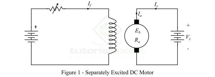
The speed of a separately excited DC motor depends upon the supply voltage and field current, i.e. magnetic flux in the machine. However, the separately excited DC motors are rarely used in practical applications because these require an external source of DC power for field excitation.
Self-Excited DC Motors
The type of DC motor whose magnetic field winding is excited from the same power supply from which the armature is supplied, is known as a self-excited DC motor.
Depending upon the manner in which the field winding is connected with the armature winding, self-excited DC motors are classified in the following three types −
Series DC motor
Shunt DC motor
Compound DC motor
Series DC Motor
A DC motor whose field winding is connected in series with the armature winding so that whole armature current passes through the field winding is called a series DC motor. Figure-2 shows the connection diagram of a series DC motor.
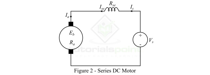
In case of a series DC motor, the field winding carries the whole armature current, thus it is made up of thick wire with less number of turns so that it possesses minimum resistance.
The following are some important expressions for the series DC motor −
$$\mathrm{\mathrm{Armature\:current},\mathit{I_{a}}\:=\:\mathit{I_{se}}\:=\:\mathit{I_{s}}}$$
Where, $\mathit{I_{se}}$ is the series field current and $\mathit{I_{s}}$ is the supply current.
$$\mathrm{\mathrm{Supply\:voltage},\mathit{V_{s}}\:=\:\mathit{E_{b}+I_{a}\left ( \mathit{R_{a}+R_{se}} \right )}}$$
Where, $\mathit{E_{b}}$ is the back EMF, $\mathit{R_{a}}$ is the armature circuit resistance, $\mathit{R_{se}}$ is the series field resistance.
Shunt DC Motor
A DC motor whose field winding is connected in parallel with the armature winding so that total supply voltage is applied across it, is known as a shunt DC motor. Figure-3 shows the connection diagram of a shunt DC motor.

In a shunt DC motor, the shunt field winding has a large number of turns of thin wire so that it has high resistance, and therefore only a part of supply current flows through it and the rest flows through the armature winding.
Following are the important expressions of a shunt DC motor −
$$\mathrm{\mathrm{Armature\:current,}\mathit{I_{a}}\:=\:\mathit{I_{s}-I_{sh}}}$$
$$\mathrm{\mathrm{Shunt\:field\:current,}\mathit{I_{sh}}\:=\:\mathit{\frac{V_{s}}{R_{sh}}}}$$
$$\mathrm{\mathrm{Supply\:Voltage,}\mathit{V_{s}}\:=\:\mathit{E_{b}+I_{a}R_{a}}}$$
Compound DC Motor
A compound DC motor is one which has two sets of field windings on each magnetic pole one is in series and the other is in parallel with the armature winding.
Compound DC motors are sub-divided into the following two types −
Short-shunt compound DC motor
Long-shunt compound DC motor
A short-shunt compound DC motor is one in which only shunt field winding is in parallel with the armature winding as shown in Figure-4.
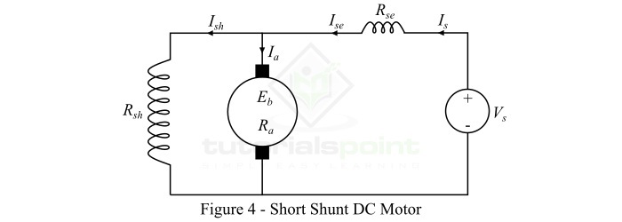
A long-shunt compound DC motor is one in which shunt field winding is in parallel with both series field winding and armature winding as shown in Figure-5.
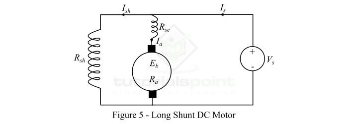
The following are the important expressions for compound DC motors −
For short-shunt motor,
$$\mathrm{\mathrm{Armature\:current,}\mathit{I_{a}}\:=\:\mathit{I_{s}-I_{sh}}}$$
$$\mathrm{\mathrm{Series\:field\:current,}\mathit{I_{se}}\:=\:\mathit{I_{a}}}$$
$$\mathrm{\mathrm{Shunt\:field\:current,}\mathit{I_{sh}}\:=\:\frac{\mathit{V_{s}}-\mathit{I_{se}R_{se}}}{R_{sh}}}$$
$$\mathrm{\mathrm{Supply\:voltage},\mathit{V_{s}}\:=\:\mathit{E_{b}+I_{a}R_{a}+I_{se}R_{se}}}$$
For long-shunt motor,
$$\mathrm{\mathrm{Armature\:current,}\mathit{I_{a}}\:=\:\mathit{I_{s}-I_{sh}}}$$
$$\mathrm{\mathrm{Series\:field\:current,}\mathit{I_{se}}\:=\:\mathit{I_{s}}}$$
$$\mathrm{\mathrm{Shunt\:field\:current,}\mathit{I_{sh}}\:=\:\frac{\mathit{V_{s}}}{R_{sh}}}$$
$$\mathrm{\mathrm{Supply\:voltage},\mathit{V_{s}}\:=\:\mathit{E_{b}+I_{a}\left ( R_{a}+R_{se} \right )}}$$
Losses in DC Machines
In DC machines (generator or motor), the losses may be classified into three categories namely,
Copper losses
Iron or core losses
Mechanical losses
All these losses appear as heat and hence raise the temperature of the machine. They also reduce the efficiency of the machine.
Copper Losses
In dc machines, the losses that occur due to resistance of the various windings of the machine are called copper losses. The copper losses are also known as I2R losses because these losses occur due to current flowing through the resistance of the windings.
The major copper losses that occur in dc machines are as,
$$\mathrm{\mathrm{Armature\:copper\:loss}\:=\:\mathit{I_{a}^{\mathrm{2}}R_{a}}}$$
$$\mathrm{\mathrm{Series\:field\:copper\:loss}\:=\:\mathit{I_{se}^{\mathrm{2}}R_{se}}}$$
$$\mathrm{\mathrm{Shunt\:field\:copper\:loss}\:=\:\mathit{I_{sh}^{\mathrm{2}}R_{sh}}}$$
In dc machines, there is also a brush contact loss due to brush contact resistance. In practical calculation, this loss is generally included in armature copper loss.
Iron Losses
The iron losses occur in core of the armature of a DC machine due to rotation of the armature in the magnetic field. Because these losses occur in core of the armature, these are also called core losses.
There are two types iron or core losses namely hysteresis loss and eddy current loss.
Hysteresis Loss
The core loss that occurs in core of the armature of a dc machine due to magnetic field reversal in the armature core when it passes under the successive magnetic poles of different polarity is called hysteresis loss. The hysteresis loss is given by the following empirical formula,
$$\mathrm{\mathrm{Hysteresis\:loss,}\mathit{P_{h}}\:=\:\mathit{k_{h}B_{max}^{\mathrm{1.6}}fV}}$$
Where, $\mathit{k_{h}}$ is the Steinmetzs hysteresis coefficient, $\mathit{B_{max}}$ the maximum flux density,f is the frequency of magnetic reversal, and V is the volume of armature core.
The hysteresis loss in dc machines can be reduced by making the armature core of such materials that have a low value of Steinmetzs hysteresis coefficient like silicon steel.
Eddy Current Loss
When the armature of a DC machine rotates in the magnetic field of the poles, an EMF is induced in core of the armature which circulates eddy currents in it. The power loss due to these eddy currents is known as eddy current loss. The eddy current loss is given by,
$$\mathrm{\mathrm{Eddy\:current\:loss,}\mathit{P_{e}}\:=\:\mathit{k_{e}B_{max}^{\mathrm{2}}f^{\mathrm{2}}t^{\mathrm{2}}V}}$$
Where,$\mathit{K_{e}}$ is a constant of proportionality, and tis the thickness of lamination.
From the expression for eddy current loss it is clear that the eddy current loss depends upon the square of thickness of lamination. Therefore, to reduce this loss, the armature core is built up of thin laminations that are insulated from each other by a thin layer of varnish.
Mechanical Losses
The power losses due to friction and windage in a dc machine are known as mechanical losses. In a dc machine, the friction loss occurs in form of bearing friction, brush friction, etc. while the windage loss occurs due to air friction of rotating armature.
The mechanical losses depend upon the speed of the machine. But these losses are practically constant for a given speed.
Note− Iron or core losses and mechanical losses together are known as stray losses.
Constant and Variable Losses
In DC machines, we may group the above discussed losses in the following two categories −
Constant Losses
Variable Losses
Those losses in a DC machine that remain constant at all loads are called constant losses. These losses include − iron losses, shunt field copper loss, and mechanical losses.
Those losses in a DC machine that vary with load are known as variable losses. The variable losses in a DC machine are − armature copper loss and series field copper loss.
Total losses in a DC machine = Constant losses + Variable losses
Applications of DC Machines
At present, a large amount of electrical energy is generated in the form of alternating current. Consequently, the use of DC machines (motors or generators) has become limited. However, dc machines are still used in several applications like for supplying excitation systems of alternators, in electrolytic processes, welding processes, etc.
Applications of DC Generators
The applications of different kinds of DC generators are listed below −
Separately-Excited DC Generator
Generators are mainly used in laboratories for experiments and testing purposes.
They are also used as a source of DC power for supplying DC motors.
Series DC Generator
Series DC generators are used in DC locomotives for regenerative braking for supplying field excitation current.
Series DC generators are also used as a booster in distribution systems.
Differentially compounded series generators are used for arc welding.
Over compounded cumulative series generators are used for lighting and heavy power supplies.
Flat compounded series generators are used for supplying power to offices, houses, and the other commercial buildings.
Shunt DC Generator
Shunt DC generators are mainly used for lighting purposes.
Shunt DC generators are used for charging batteries.
These generators are also used for supplying field excitation current to alternators.
Applications of DC Motors
The applications of different types of DC motors are given below −
Series DC Motor
Series DC motors are used in applications where high starting torque is required.
Series DC motors are used in cranes and hoists.
Series DC motors are used in electric tractions.
They are used in air compressors.
They are also used in vacuum cleaners.
Series DC motors are also used in sewing machines, etc.
Shunt DC Motor
Shunt DC motors are used in applications that require constant speed.
Shunt DC motors are used for driving lathe machines.
These are also used in centrifugal pumps and blowers.
These are used in fans, conveyors, and spinning machines.
These DC motors are also used in lifts.
Compound DC Motor
Compound DC motors are used in those applications which require high starting torque and constant speed.
Used in printing presses.
They are also used in shears.
They are used in elevators and lifts.
Compound DC motors are also used in rolling mills and heavy planners, etc.
Introduction to Induction Motor
Induction motors are the most widely used electric motors in industrial applications. Almost all induction motors run at essentially constant speed from no-load to full-load conditions. The speed of induction motors depends on the supply frequency and hence these motors are not easily adapted to speed control. Induction motors are simple and rugged in construction, less expensive, easy to maintain, and can be designed and produced with characteristics to suit most industrial requirements.
What is an Induction Motor?
An induction motor is an asynchronous AC electric motor which converts alternating current electricity into the mechanical energy. It is called an induction motor because the electric current in the rotor circuit required to produce the deriving torque is obtained through electromagnetic induction from the rotating magnetic field of the stator winding.
These motors are referred to as asynchronous motors because their rotor rotates at a speed less than the synchronous speed of the rotating magnetic field.

The induction motor is an electromechanical energy conversion device, i.e. it converts electrical energy into mechanical energy in the form of rotation of shaft. Like any electric motor, an induction motor has two main parts namely stator and rotor.
The stator carries a set of windings called stator winding. The stator winding may be single-phase winding or three-phase winding.
The rotor carries a short-circuited winding called rotor winding.
In case an induction motor, only the stator winding is fed from an AC supply, while the rotor winding derives its voltage and power from the stator winding through electromagnetic induction.
Working Principle of Induction Motor
The working of an induction motor is based on the principle of electromagnetic induction. In an induction, there are two windings namely, stator winding and rotor winding. The input AC supply is connected to the stator winding, the current flowing in the stator winding produces a magnetic flux. This magnetic flux is usually rotating, hence also called rotating magnetic field. The rotor winding of the induction motor is a short-circuit winding.
The rotating magnetic flux from the stator cuts the short-circuited conductors of the rotor winding. According to Faradays law of electromagnetic induction, an EMF is induced in the rotor circuit which causes a current to flow through it. When the current flows through the rotor winding, another magnetic flux being produced in the machine.
Therefore, there are two magnetic fluxes inside the induction motor, one is stator flux and the other is rotor flux. These two magnetic fluxes interact with each other. Because of that, the rotor will experience a torque which makes the rotor to rotate in the direction of the rotating magnetic field of the stator. In this way, an induction motor runs.
Types of Induction Motors
Depending on the type of input supply, induction motors are classified into the following two types −
Single-Phase Induction Motors− An induction motor that works on single-phase AC supply is called as a single-phase induction motor.
Three-Phase Induction Motors− An induction motor which requires three-phase AC supply to operate is called a three-phase induction motor.
Advantages of Induction Motors
The following are some major advantages of induction motors −
Induction motors have simple and rugged construction.
Induction motors are relatively less expensive.
Induction motors have relatively high efficiency.
Induction motors can be designed to have characteristics to meet the industrial requirements.
Induction motors need little maintenance.
Disadvantages of Induction Motors
The main disadvantages of induction motors are as follows −
The speed of induction motors cannot be changed easily because they are essentially constant speed motors.
Induction motors draw a high inrush current at starting.
Induction motors always operate at lagging power factor.
Single-phase induction motors are not self-starting; hence we need provide some extra starting mechanism.
Single-Phase Induction Motor
As the name implies, these induction motors are operated on a single-phase AC supply. Single-phase induction motors are the most familiar electric motors because these are commonly used in domestic and commercial appliances like fans, pumps, washing machines, air conditioners, refrigerators, etc.
Although single-phase induction motors are relatively less efficient than three-phase induction motors, but they are extensively used as the substitute for three-phase induction motors in low power applications.
A typical single-phase induction motor consists of two main parts − a stator and a rotor. The stator of a single-phase induction motor carries a single-phase winding, whereas the rotor has the squirrel-cage construction.
How to Make an Induction Motor Self Start?
The major drawback of a single-phase induction motor is that it is not self-starting, but requires some starting mechanism. In single-phase induction motors, the stator winding produces a pulsating magnetic field which varies in sinusoidal manner. Hence, this magnetic field reverses its polarity after each half-cycle of AC, but does not rotate in space. As a result, this alternating magnetic field does not produce rotation in a stationary rotor. Although, if the rotor is rotated in one direction by some external mean, it will continue to run in the direction of rotation. However, this method of starting a single-phase induction motor is not convenient in practice.
Therefore, in order to make a single-phase induction motor self-starting, we are somehow required to produce a revolving magnetic field inside the motor. This can be achieved by converting a single-phase AC supply into two-phase AC supply by providing an additional winding. Thus, a single-phase induction motor consists of two windings on its stator, namely main winding and starting winding. These windings are 90 out of phase with each other.
Types of Single-Phase Induction Motors
Depending upon the method employed to make the motor self-starting, single-phase induction motors may be classified into the following three types −
Split-phase induction motor
Capacitor-start induction motor
Capacitor-start capacitor-run induction motor
Let us now discuss each of these Induction Motors in greater detail.
Split-Phase Induction Motor
A split-phase induction motor is a type of single-phase induction motor in which the stator consists of two windings namely, a starting winding and a main winding, where the starting winding is displaced by 90 electrical from the main winding.
The starting winding operates only during the starting period of the motor. The starting and main windings are so designed that the starting winding has high resistance and relatively low reactance, while the main winding has relatively low resistance and high reactance so that currents flowing in the two windings have a reasonable phase difference ($\alpha$) of about 25 to 30.
Now, when the starting winding of the motor is connected to a source of single-phase ac supply, the starting winding carries a current $\mathit{I_{s}}$, while the main winding carries a current $\mathit{I_{m}}$ as shown in Figure-1.
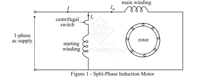
As the starting winding is made highly resistive whereas the main winding highly inductive. Consequently, the currents $\mathit{I_{s}}$ and $\mathit{I_{m}}$ in the two windings have a reasonable phase difference of about 25 to 30. As a result, a weak revolving magnetic field is produced inside the motor which starts it.
Capacitor Start Induction Motor
The type of single-phase induction motor in which a capacitor C is connected in series with the starting winding as shown in Figure-2. This capacitor is called starting capacitor. The value of starting capacitor is so chosen that the starting current $\mathit{I_{s}}$ leads the current $\mathit{I_{m}}$ through the main winding by about 80.
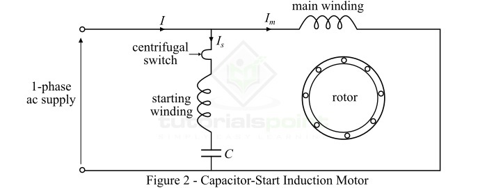
Once the motor attains about 75% of the rated speed, a centrifugal switch isolates the starting winding from the circuit. The motor then operates as a single-phase induction motor and continues to accelerate till it reaches the normal speed. Therefore, in this type of single-phase induction motor, the capacitor in series with the starting winding introduces a phase shift between the two windings so that the motor can start itself.
Capacitor-Start Capacitor Run Induction Motor
This motor is almost identical to a capacitor-start induction motor except that the starting winding is not disconnected from the motor circuit. Therefore, in case of capacitor-start capacitor-run induction motor, both the windings (starting winding & main winding) remain connected to the supply during starting as well as running period.
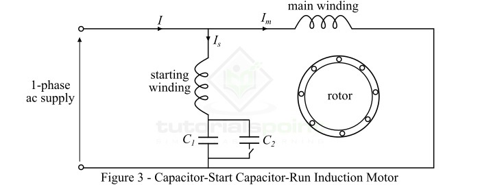
In this motor, two capacitors C1 and C2 are used in the starting winding as show in Figure-3. The capacitor C1 having small capacitance value is used for optimum running of the motor and hence permanently connected in series with the starting winding, whereas the larger capacitor C2 is connected in parallel with C1 and it remains in the circuit during starting period only. The starting capacitor C2 is isolated from the circuit by a centrifugal switch when the motor reaches about 75% of rated speed. The motor is then runs as a single-phase induction motor.
Applications of Single-Phase Induction Motors
Single-phase induction motors are mainly used in domestic and commercial appliances like fans, ACs, refrigerators, air-cooler, washing machines, etc. Given below are some of the applications of different kinds of single-phase induction motors −
Split-Phase Induction Motors − These motors are best suited for moderate starting-torque applications like fans, washing machines, oil burners, small machine tools, etc.
Capacitor-Start Induction Motors − These motors are suitable for applications that require relatively high-starting torque like compressors, large fans, pumps and high-inertia loads, etc.
Capacitor-Start Capacitor-Run Induction Motors − These motors are suitable for constant torque, and vibration free applications like in hospital appliances, studio equipment and in many other appliances that are used in such areas where silence is important.
Three-Phase Induction Motor
As the name suggests, a three-phase induction motor is one which works on three-phase AC supply, and converts three-phase AC electricity into mechanical energy. Three-phase induction motors are the most extensively used electric motors in industries. These motors run at almost a constant speed from no-load to full-load, i.e., they have good speed regulation. Although the speed of three-phase induction motors depends on the supply frequency and number of poles in the machine and therefore, it is quite difficult to change their speed.
Just like any other electric motor, a typical three-phase induction motor also consists of two main parts namely stator and rotor. The stator is a stationary part and carries a three-phase winding, called stator winding. The rotor is a rotating part of the motor and carries a short-circuited winding, called rotor winding.
The stator winding of a three-phase induction motor is fed from a three-phase balanced AC supply, while the rotor winding derives its working voltage and power from the stator winding via electromagnetic induction. This is why, it is named so.
A three-phase induction motor may be considered to be a three-phase transformer with a rotating secondary winding. Therefore, it could be described as a transformer-type AC machine. The only difference is that the induction motor converts electricity into mechanical energy.
Types of Three-Phase Induction Motors
According to the rotor construction, three-phase induction motors are classified into the following two basic types −
Squirrel-Cage Induction Motor
Slip-Ring Induction Motor
Advantages of Three-Phase Induction Motors
Here is a list of some of the major advantages of three-phase induction motors −
The design and construction of three-phase induction motors are quite simple.
They have robust construction.
Three-phase induction motors require less maintenance.
Three-phase induction motors have self-starting property.
These motors have reasonably good power factor.
Three-phase induction motors are more economical.
They have high efficiency.
Disadvantages of Three-Phase Induction Motors
The major disadvantages of three-phase induction motors are listed below −
Three-phase induction motors are essentially constant speed motors, and require complex mechanism to change the speed.
Three-phase induction motors always work on lagging power factor.
These motors draw very high starting current.
Applications of Three-Phase Induction Motors
The major applications of three-phase induction motors are given below −
The squirrel-cage type three-phase induction motors are suitable for driving blowers, fans, machine tools, centrifugal pumps, etc.
Three-phase induction motors are also used for driving different industrial load like compressors, crushers, conveyors, reciprocating pumps, etc.
The slip-ring induction motors are best suited for driving loads that require high starting toque like crushers, plungers, cranes, elevators, hoists, conveyors, etc.
Construction of Three-Phase Induction Motor
A three-phase induction motor consists of two main parts namely,
Stator
Rotor
There is a small air gap between the stator and rotor which ranges from 0.4 mm to 4 mm depending on the power rating of the motor.
Stator
The stator of a three-phase induction motor is a stationary part, and it consists of a cylindrical-shaped frame made up of fabricated steel. This steel frame encloses a hollow cylindrical core made up of thin laminations of silicon steel. On the inner periphery of the core, a number of evenly spaced slots are provided to place the stator winding. The silicon-steel laminations are used to reduce the hysteresis and eddy current losses.
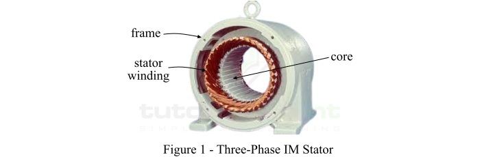
Three windings are placed in the stator slots and are suitably connected to form a balanced three-phase delta or star connected circuit. As per the requirement of motor speed, these three-phase windings are wound for a definite number of poles. Where, greater is the number of poles, lesser is the speed of the induction motor and vice-versa.
When we fed the three-phase stator winding from a balanced three-phase supply, a rotating magnetic field of constant magnitude is produced. This rotating magnetic induces EMF in the rotor circuit by electromagnetic induction.
Rotor
The rotor is a rotating or moving part of the three-phase induction motor. It consists of a rotor core made up of thin laminations of high grade silicon steel to reduce the hysteresis and eddy-current losses. The rotor core is a hollow cylinder, mounted on a shaft. On outer periphery of the rotor core, slots are provided to place the rotor winding.
Based on the construction, the rotor of a three-phase induction motor can be of the following two types −
Squirrel-cage rotor
Wound rotor
Let's discuss these two types of rotors in detail.
Squirrel Cage Rotor
The squirrel-cage rotor consists of a laminated cylindrical core having parallel slots on its outer periphery. In case of squirrel-cage rotor, the rotor winding is made up of metal (copper or aluminium) bars. These metal bars are placed in the rotor slots and are short-circuited at each end by metal rings called end-rings as shown in Figure-2.
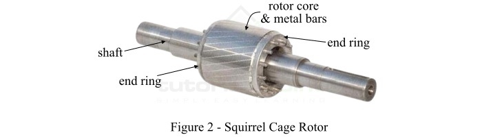
From Figure-2, it can be observed that the construction of this rotor resembles a squirrel cage and hence the name. Here, it is also to be noted that the rotor is not connected electrically to the supply, but it derives its voltage and power by the electromagnetic induction from the stator.
The three-phase induction motors that employ squirrel-cage rotor are known as squirrel-cage induction motors. Almost 70% to 80% three-induction motors used in industrial applications are squirrel-cage induction motors because of their simple and robust construction which enable them to operate in most adverse circumstances. Although, the induction motors that use squirrel-cage rotor have a low starting torque.
Wound Rotor
The wound rotor consists of a laminated cylindrical core made up of silicon steel. It carries a 3-phase rotor winding similar to the stator winding as shown in Figure-3.

The rotor winding of the wound rotor is uniformly distributed in the slots and is connected in star fashion. The open ends of the star-connected rotor winding are brought out and connected to three slip rings mounted in the rotor shaft. A carbon brush is resting on each slip ring, and through these brushes, external resistances can be added to the rotor circuit.
At starting, suitable values of external resistances are added into phases of the rotor winding to obtain a high starting torque. These external resistances are gradually removed from the circuit as the motor runs up to speed. The use of external resistances considerably reduces the starting current and increases the starting torque of the motor. Once the motor attains normal speed, the three carbon brushes are short-circuited so that the wound motor runs like a squirrel cage induction motor.
Three-Phase Induction Motor on Load
In this chapter, we will explain the behavior of a three-phase induction motor on load.
When we attach a mechanical load to the rotor shaft of the three-phase induction motor, it will begin to slow down and thus the rotating magnetic field (RMF) will cut the rotor conductors at a higher rate. Because of this, the induced EMF and resulting current in the rotor conductors will increase gradually, and producing a higher torque. This torque accelerates the rotor, and the rotor and mechanical load will soon reach a state of equilibrium when the rotor torque and load torque become equal. Once this state is reached, the speed of the motor stops to decrease further, and hence the motor will run at the new speed at a constant rate.
However, the decrease in speed of a three-phase induction motor with increased load is small. It is because, impedance of its rotor circuit is low, and a small drop in the speed produces a large rotor current. This increased rotor current produces a higher torque to meet the increased load demand on the motor shaft. This is why the 3-phase induction motors are considered to be constant speed motors. However, these motors never run at synchronous speed, thus they are also called asynchronous motors.
Technically, the change in load on the three-phase induction motor is met through the adjustment of slip (difference of synchronous speed and rotor speed). Which means, the slip increases slightly with the increase in load on the motor shaft. Due to this, the relative speed between the rotating magnetic field and rotor conductors is increased. Consequently, the rotor current is increased, producing a higher motor torque to meet the increased load demand.
Also, with increasing mechanical load, the increased rotor current is in such a direction so as to decrease the rotating magnetic flux of the stator (according to Lenzs law), thus decreasing the back EMF in the stator windings. The decreased back EMF allows the stator current to increase, and hence increasing the power input to the induction motor.
Concept of Slip in Induction Motor
In a three-phase induction motor, the rotor can never reach the speed of stators rotating magnetic field (called synchronous speed). If it did, there would be no relative motion between the rotating magnetic field and rotor conductors, no induced EMF in the rotor conductors, and hence no torque to rotate the rotor. Therefore, in practice, the speed of rotor of an induction motor is always less than the synchronous speed. This difference is known as slip speed, i.e.,
$$\mathrm{\mathrm{Slip\:speed}\:=\:\mathit{N_{s}-N_{r}}}$$
Where, $\mathit{N_{s}}$ is the synchronous speed and $\mathit{N_{r}}$ is the rotor speed.
$$\mathrm{\mathrm{Synchronous\:speed,}\mathit{N_{s}}\:=\:\frac{120\mathit{f}}{\mathit{P}}}$$
Where,f is the supply frequency and P is the number of poles in induction motor.
The ratio of the slip speed to the synchronous speed is called the slip of the induction motor, i.e.,
$$\mathrm{\mathrm{Slip,}\mathit{s}\:=\:\frac{\mathit{N_{s}-N_{r}}}{\mathit{N_{s}}}}$$
Also,
$$\mathrm{\mathrm{Percentage\:Slip,}\mathit{s}\:=\:\frac{\mathit{N_{s}-N_{r}}}{\mathit{N_{s}}}\times 100\%}$$
In a practical three-phase induction motor, the change in the slip from no-load to full-load is around 0.1% to 3%.
Numerical Example
An 8-pole 3-phase induction motor is connected to a 60 Hz supply. If it is running at 880 RPM. Calculate the slip.
Solution
Given data,
Poles,P = 8
Frequency,f = 60 Hz
Rotor speed,Nr= 880 RPM
$$\mathrm{\therefore \mathrm{Synchronous\:speed,}\mathit{N_{s}}\:=\:\frac{120\times 60}{8}\:=\:900}$$
Therefore, the slip will be,
$$\mathrm{\mathrm{Slip,}\mathit{s}\:=\:\frac{900-880}{900}\times 100\:=\:2.22\%}$$
Characteristics of 3-Phase Induction Motor
The operating performance of a three-phase induction motor can be explained with the help of the following two characteristics namely,
Torque-Slip Characteristics
Torque-Speed Characteristics
Torque Slip Characteristics of 3 Phase Induction Motor
The torque-slip characteristics of a three-phase induction motor is the curve drawn between the motor torque and slip for a particular value of rotor resistance. Figure-1 shows different torque-slip characteristics of a typical three-phase induction motor for a slip range from s = 0 to s= 1 for various values of rotor resistance.
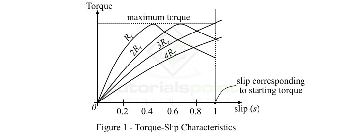
For a three-phase induction motor, the relation between the motor torque and slip under running condition is given by,
$$\mathrm{\mathit{\tau _{r}}\:=\:\frac{\mathit{KsR_{r}}}{\mathit{R_{r}^{\mathrm{2}}+s^{\mathrm{2}}X_{r}^{\mathrm{2}}}}\:\cdot \cdot \cdot (1)}$$
Where,K is a constant,s is the slip, $\mathit{R_{r}}$ is the per phase rotor resistance, and $\mathit{X_{r}}$ is the standstill rotor reactance per phase.
From Equation-1, we may conclude the following points −
Case 1
If s = 0, then $\mathit{\tau _{r}}\:=\:0$. Therefore, the torque-slip curve starts from the origin.
Case 2
At normal speed of the motor, the slip is small, and thus $\mathit{sX_{r}}$ is practically negligible as compared to $\mathit{R_{r}}$.
$$\mathrm{\therefore \mathit{\tau _{r}}\propto \mathit{\frac{s}{R_{r}}}}$$
Since for a given motor, $\mathit{R_{r}}$ is also constant.
$$\mathrm{\therefore \mathit{\tau _{r}}\propto \mathit{s}}$$
Thus, the torque-slip curve is a straight line from zero slip to a slip that corresponds to full load.
Case 3
If slip value exceeds the full-load slip, then torque increases and becomes maximum when $\mathit{R _{r}}\:=\:\mathit{s\:X_{r}}$. This maximum torque in a three-phase induction motor is known as breakdown torque or pull-out torque. The value of the breakdown torque is at least double of the full-load torque when the induction motor is operated at rated voltage and frequency.
Case 4
When the slip value becomes greater than that corresponding to the maximum torque, then the term $\mathit{s^{\mathrm{2}}\:X_{r}^{\mathrm{2}}}$ increases rapidly so that $\mathit{R_{r}^{\mathrm{2}}}$ may be neglected.
$$\mathrm{\therefore \mathit{\tau _{r}}\propto \mathit{\frac{s}{s^{\mathrm{2}}X_{r}^{\mathrm{2}}}}}$$
As $\mathit{X_{r}^{\mathrm{2}}}$ is practically constant, then
$$\mathrm{\mathit{\tau _{r}}\propto \mathit{\frac{\mathrm{1}}{s}}}$$
Hence, the torque is now inversely proportional to the slip. Thus, the torque-slip curve is a rectangular hyperbola.
Therefore, from the above analysis of torque-slip characteristics of a three-phase induction motor it is clear that the addition of resistance to the rotor circuit does not change the value of maximum torque, but it only changes the value of slip at which the maximum torque occurs.
Torque-Speed Characteristic of 3-Phase Induction Motor
For a three-phase induction motor, the motor torque depends upon the speed but we cannot express the relationship between them by a simple mathematical equation. Therefore, we use a torque-speed characteristic curve to show this relationship. Figure-2 shows a typical torque-speed characteristic curve of a three-phase induction motor.
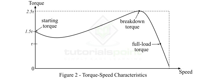
The following points may be noted from this characteristic curve −
If the full-load torque is $\tau$, then the starting torque is $1.5\tau $ and the maximum torque (or breakdown torque) is $2.5\tau $
At full-load, if speed of the motor is N, and if the mechanical load on the shaft increases, the speed of the motor will drop until the motor torque is again equal to the load torque. Once the two torques are equal, the motor will run at a constant speed but lower than the previous. Although, if the motor torque becomes greater than $2.5\tau $(i.e. breakdown torque), the motor will suddenly stop.
For a three-phase induction motor, the torque-speed curve is essentially a straight line between the points of no-load and full-load. The slope of the curve line depends upon the resistance of the rotor circuit, i.e., greater the resistance, the sharper the slope.
Speed Regulation and Speed Control
Speed Regulation of Induction Motors
The speed regulation of induction motor is defined as the change in the motor speed with change in load. It is expressed as a fraction or percentage of full-load speed, i.e.,
$$\mathrm{\mathrm{Speed\:regulation}\:=\:\mathit{\frac{N_{nl}-N_{fl}}{N_{fl}}}\times 100\%}$$
Where,$\mathit{N_{nl}}$ is the no-load speed of the motor and $\mathit{N_{fl}}$ is the full-load speed of the motor.
The speed regulation of an induction motor is about 3% to 5%. Due to this small speed regulation, the induction motors are classified as the constant speed motors.
Speed Control of Three-Phase Induction Motors
The speed of a three-phase induction motor is given by,
$$\mathrm{\mathit{N_{r}}\:=\:\left ( 1-\mathit{s} \right )\mathit{N_{s}}\:\cdot \cdot \cdot (1)}$$
Where,s is the slip and $\mathit{N_{s}}$ is the synchronous speed in RPM.
$$\mathrm{\mathit{N_{s}}\:=\:\frac{120\mathit{f}}{\mathit{P}}\:\cdot \cdot \cdot (2)}$$
From equations (1) & (2), it is clear that the speed of a three-phase induction motor can be varied by changing the following −
Frequency (f) of AC supply,
Number of stator poles (P), and
Slip (s).
In practice, the change in supply frequency is generally not possible because the commercial electric supplies have a constant frequency. Hence, the speed of a three-phase induction motor can be changed either by changing the number of stator poles (P) or the slip (s). We shall now discuss the speed control of squirrel-cage and slip-ring induction motors.
Speed Control of Squirrel-Cage Induction Motors
The speed control of squirrel-cage induction motors is changed by changing the number of stator poles. By the pole changing method, there are only two or four speeds are possible.
In a two-speed induction motor, one stator winding is provided, which may be switched through a suitable control equipment to provide the two speeds. Where, one speed is half of the other. For example, the stator winding may be connected for either 4 or 8 stator poles, giving synchronous speeds of 1500 RPM and 750 RPM, when the motor is supplied from a source of 50 Hz AC supply.
In a four speed induction motor, two separate stator windings are provided each of which provides two speeds.
Following are the major disadvantages of pole changing method of speed control −
This method cannot be used to obtain gradual continuous speed control.
It makes the motor design and switching of the interconnection of stator windings more complicated.
This method can provide a maximum of four different speeds for any one motor due to design and interconnection complications.
Speed Control of Slip-Ring Induction Motors
The speed of a slip-ring induction motor can be varied by changing the motor slip. The following methods are employed for changing the slip and hence the speed −
By the changing the stator line voltage.
By changing the resistance of the rotor circuit.
By adding and changing a foreign voltage in the rotor circuit.
Numerical Example
For a three-phase induction motor, the no-load speed of the motor is 900 RPM and its full-load speed is 880 RPM. Find the speed regulation of the motor.
Solution
Given data,
$\mathit{N_{nl}}$ = 900 RPM
$\mathit{N_{fl}}$ = 880 RPM
$$\mathrm{\therefore\mathrm{Speed\:regulation}\:=\:\mathit{\frac{N_{nl}-N_{fl}}{N_{fl}}}\times 100\%}$$
$$\mathrm{\Rightarrow \mathrm{Speed\:regulation}\:=\:\frac{900-880}{880}\times 100\%\:=\:2.273\%}$$
Methods of Starting 3-Phase Induction Motors
The following four methods are extensively used for starting the three-phase induction motors −
Direct-On-Line Starter
Auto-Transformer Starter
Star-Delta Starter
Rotor Resistance Starter
In this chapter, let's discuss each of these starting methods in detail.
Direct On Line Starter
As the name implies, the direct-on line (D.O.L.) starter is one in which the three-phase induction motor is started by connecting it directly to a 3-phase balanced ac supply as shown in Figure-1.
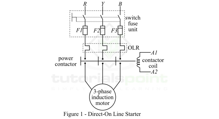
In this method, the induction motor draws a very high starting current about 4 to 10 times of the full-load current. It is because, the impedance of the motor at standstill is low. Therefore, the direct-on line (D.O.L.) method of starting is suitable for the motor of low power rating, usually up to 7.5 kW.
Autotransformer Starter
In this method of induction motor starting, a three-phase autotransformer is used to supply three-phase electricity to the motor. The autotransformer is mainly used to reduce the 35. Methods of Starting 3-Phase Induction Motors supply voltage at starting and then connecting the motor to the full supply voltage as the motor attains a sufficient speed.
The circuit arrangement of autotransformer starter is shown in Figure-2. The tapings on the autotransformer used for starting the induction motors are provided in such a way that when it is connected in the circuit, 60% to 80% of the supply voltage is applied to the motor.
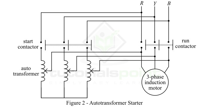
At the instant of starting, the autotransformer is put into the circuit and hence reduced voltage is applied to the motor. Consequently, the starting current is limited to a safe value. When the motor reaches about 80% of the rated speed, the autotransformer is removed from the circuit through a changeover switch, and the motor is then connected to the full supply voltage. The autotransformer starter has several advantages like low power loss, small starting current, etc. Therefore, this method is suitable for relatively larger induction motors of power ratings over 25 hp.
Star-Delta Starter
In this method, the three-phase induction motor is started as a star-connected motor and run as a delta-connected motor.
The induction motors which are started by star-delta starter has the stator windings which are designed for delta operation and are connected in star during the starting period. When the motor attains a sufficient speed, the winding connections are changed from star to delta.
Figure-3 shows the circuit arrangement of the star-delta starter. Here, the six terminals of the stator windings are connected to a changeover switch. At the instant of starting, the changeover switch connects the stator windings in star-configuration. As a result, each stator phase gets a voltage equal to V/3, where V is the full line voltage. In this way, the stator windings get a reduced voltage during starting period.
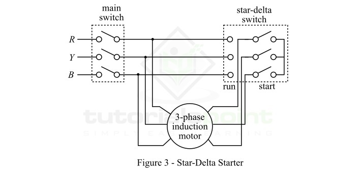
When the motor attains a specific speed, the changeover switch turns the connection of stator windings to delta. Each phase now gets the full line voltage V, and the motor runs at the normal speed. However, this method of starting of three-phase induction motor causes a large reduction in the starting torque of the motor. This method is best suited for medium sized induction motors, up to about 25 hp.
Rotor Resistance Starter
This method of starting is applicable to slip-ring induction motors only. In this method, a variable star-connected rheostat is inserted into the rotor circuit through slip rings, and full supply voltage is applied to the stator winding. The circuit arrangement of rotor resistance starter is shown in Figure-4.
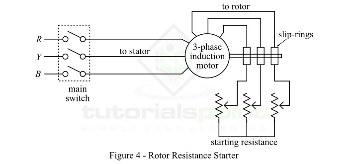
At the instant of starting, the handle of the star-connected rheostat is set in the off position. Consequently, a maximum resistance is inserted in each phase of the rotor circuit, and reduces the starting current. At the same time, this resistance increases the starting torque.
When the motor picks up speed, the external resistance is gradually removed from the rotor circuit by moving the rheostat handle. Once the motor attained about 80% of the normal speed, the handle is switched to the on position, and thus the whole external resistance is removed from the rotor circuit.
Introduction to 3-Phase Synchronous Machines
An electromechanical energy conversion device (or electrical machine) which operates on synchronous speed (i.e. speed of rotating magnetic field) is termed as a synchronous machine. A synchronous machine an AC machine, i.e., it requires AC supply to work.
Based on the energy conversion, synchronous machines may be classified into two types −
Synchronous Generator
Synchronous Motor
The synchronous machines are the most extensively used electrical machines in power system applications like power generator, power factor correction, driving constant speed mechanical load, etc.
The synchronous machine which converts mechanical energy into alternating current electricity is called a synchronous generator or alternator. While the synchronous machine which converts alternating current electricity into mechanical energy is called a synchronous motor.
The synchronous machines, used in most practical applications, are three-phase AC machines. However, there are single-phase synchronous machines also exist but they are used in special applications.
A synchronous machine (generator or motor) always operate at a constant speed called synchronous speed. The synchronous speed is given by the following relation,
$$\mathrm{\mathit{N_{s}}\:=\:\frac{120\mathit{f}}{\mathit{p}}\cdot \cdot \cdot (1)}$$
Where,
f is the supply frequency,
P is the number of poles in the machine.
The synchronous speed is measured in revolution per minute (RPM).
For satisfactory operation, a synchronous machine always maintains the expression given in Equation-1. If the synchronous machine fails to maintain the above relationship of Equation-1. The machine will stop to operated, and this condition is known as loss of synchronism or out of synchronism of the machine. Hence, this proves that the synchronous machine is designed to operate at a constant speed.
Working Principle of Synchronous Machine
The working principle of a synchronous machine is based on the law of electromagnetic interaction and law of magnetic interlocking.
According to the law of electromagnetic interaction, when there is a relative motion between a conductor and a magnetic field, an EMF is induced in the conductor. On the other hand, when a current carrying conductor is placed in a magnetic field, a force acts on the conductor that tends to move it.
According to the law of magnetic interlocking, two different magnetic fields (field of stator and field of rotor) are locked together and rotate at the same speed. This phenomenon is called magnetic interlocking.
These two principles explain the working of a synchronous machine. The synchronous machine is first started by the electromagnetic interaction, and then the magnetic fields of rotor and stator are locked together to rotate at the synchronous speed.
Three-Phase Synchronous Generator
A synchronous machine that converts mechanical energy into 3-phase electrical energy through the process of electromagnetic induction is known as a 3-phase synchronous generator or alternator.
A 3-phase alternator consists of an armature winding and a field winding, where the EMF is induced in the armature winding, while field winding produces the working magnetic field. In case of a 3-phase alternator, the armature winding is provided on the stator part of the machine while the field winding is provided on the rotor. The major advantage of stationary armature winding is that there is no need of commutator as required in the DC generators.
The 3-phase synchronous generators are most widely used for generation of electric power in power generating plants.
Three-Phase Synchronous Motor
A synchronous machine that converts three-phase electricity into mechanical energy is known as three-phase synchronous motor.
Like any other electric motor, a synchronous motor also consists of two major parts namely stator and rotor. The stator carries a three-phase armature winding, whereas the rotor carries a field winding which is excited from a dc supply to produce a certain number of fixed magnetic poles.
A unique feature of a synchronous motor is that it can run at a constant speed, called synchronous speed. Although, the major disadvantage of a three-phase synchronous motor is that it does not have self-starting torque. Therefore, in order to start a 3-phase synchronous motor, it is brought up almost to its synchronous speed by some auxiliary mean.
Being a constant speed motor, the load on the motor does not exceed the limiting value. If the load on the motor exceeds the limiting value, the motor will immediately stop. The three-phase synchronous motors are used for − driving mechanical loads at constant speed, improving power factor of a system, etc.
Features of Synchronous Machines
The following are the key features of synchronous machines (motor or generator) −
Synchronous motors do not self-starting torque.
Synchronous machine is a doubly-excited machine because it requires two input supplies one on the stator and the other on the rotor.
Synchronous machines operate at constant speed, called synchronous speed.
Synchronous generators can produce a voltage of constant magnitude and frequency.
A synchronous machine can be operated at lagging, leading or unity power factor just by changing the excitation.
Synchronous motors have relatively high starting torque as compared to induction motors.
Synchronous motors are suitable for driving constant and slow speed (usually less than 300 RPM) loads.
Synchronous machines are expensive.
Construction of Synchronous Machine
Like any other rotating electrical machine, a synchronous machine (generator or motor) has two essential parts namely,
Stator − It is a stationary part of the machine and carries the armature winding.
Rotor − It is the rotating part of the machine. The rotor of a synchronous machine produces the main field flux.
In this chapter, let's discuss how the Stator and Rotor of a Synchronous Machine is constructed.
Stator Construction
The stator of a synchronous machine includes various parts like frame, stator core, stator windings and cooling mechanisms, etc. The frame is the outer part of the machine, and made up of cast iron for small-sized machines, and of welded steel for large-sized machines. The frame encloses the whole machine assembly and protects it from mechanical and environmental impacts.

The stator core is a hollow cylinder which is made up of high-grade silicon steel laminations. The silicon steel laminations reduce the hysteresis and eddy-current losses in the machine. A number of evenly spaced slots are provided on the inner periphery of the stator core. A three-phase winding is put in these slots. When current flows through the stator winding, it produces a sinusoidal magnetic field and hence the EMF.
Rotor Construction
In synchronous machines, there are two types of rotor constructions used namely, salient-pole rotor and cylindrical rotor.
Salient-Pole Rotor
The term salient means projecting. Hence, a salient-pole rotor is one that consists of field poles projecting out from the surface of the rotor core as shown in Figure-2.

Since the rotor is subjected to a changing magnetic field, therefore it is made up of thin steel lamination to reduce the eddy current loss. The field poles of same dimensions are constructed by stacking laminations of the required length and then riveted together. After wounding the field coils around each pole core, poles are fitted to a steel spider keyed to the rotor shaft.
At the outer end of each pole, damper bars are provided to dame out the oscillations of rotor during sudden changes in the load. Though, the synchronous machines using the salient-pole rotor have a non-uniform air gap, where the air gap is minimum under the pole centers and it is maximum in between the field poles. The pole face (outer end of the pole) is so shaped that length of the radial air-gap increases from the pole center to the pole tip so it can result a sinusoidal distribution of flux in the air-gap. This will ensure the smooth operation of synchronous machine.
In the salient-pole rotor, the individual field coils are connected in series so that they can give alternate north and south poles. The ends of the field coils are connected to a source of DC supply though brushes and slip-rings.
The synchronous machines having salient-pole rotor usually have a large number of field poles, and operate at lower speeds. These machines have a larger diameter and a shorter axial-length.
Cylindrical Rotor
This type of synchronous machine rotor construction has a smooth cylindrical structure. In case of cylindrical rotor, there are no physical poles projecting outward. The cylindrical rotor is made from slid forgings of high-grade Ni-Cr-Mo steel.
On the outer periphery of the rotor, evenly spaced slots are cut in about two-third part of the rotor and theses slots are parallel to the rotor shaft. The field windings are placed in these slots. The field windings are excited from a source of DC supply. The un-slotted part of the rotor forms pole-faces.

The synchronous machines that use cylindrical rotor have a smaller diameter and longer axial length. The cylindrical rotor construction limits the effect of centrifugal forces. Consequently, the cylindrical rotor construction is mainly used in high-speed synchronous machines. Also, this rotor construction provides a greater mechanical strength and permits relatively more accurate dynamic balancing to the machine.
The major advantage of having a synchronous machine using cylindrical rotor is that it makes less mechanical losses. Since the cylindrical rotor provides a uniform air-gap in the machine, hence their operation is less noisy.
Working of 3-Phase Alternator
A 3-phase alternator is a synchronous machine that converts mechanical energy into 3-phase electrical energy through the process of electromagnetic induction.
As we discussed in previous chapters, a 3-phase alternator, also called a 3-phase synchronous generator, has a stationary armature and a rotating magnetic field. In the three-phase alternator, the rotor winding (serves as field winding) is energized from a DC supply and alternate north and south poles are developed on the rotor.
Operation of Three-Phase Alternator
When the rotor is rotated (say in anticlockwise direction) by a prime mover (engine, turbine, etc.), the stator winding (serves as armature winding) is cut by the magnetic flux of the rotor poles. Due to electromagnetic induction, an EMF is induced in the armature winding. This induced EMF is alternating one because the north and south poles of the rotor alternately pass the armature winding conductors. We can determine the direction of the induced EMF by Flemings right hand rule.
The electrical equivalent circuit of a star-connected armature winding and dc field winding three-phase alternator is shown in Figure-1.
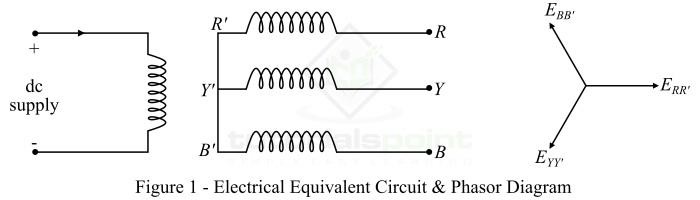
When the rotor is rotated a three-phase voltage is generated in the armature winding. The magnitude of generated voltage depends upon the speed of the rotation of rotor and the DC excitation current. However, the magnitude of generated voltage in each phase of the armature is the same, but displaced by 120 electrical from each other in space as shown in the phasor diagram.
Frequency of Generated Voltage
In a three-phase alternator, the frequency of generated voltage depends upon the speed of rotation and the number of field poles in machine.
Let
N = speed of rotation in RPM
P = number of field poles
Then, the frequency of generated voltage is given by,
$$\mathrm{\mathit{f}\:=\:\frac{\mathit{NP}}{120}\:\mathrm{Hz}\:\cdot \cdot \cdot (1)}$$
It should be noted that N is the synchronous speed because the alternator is a synchronous machine whose rotor always rotates at the synchronous speed.
EMF Equation of Three-Phase Alternator
The mathematical relation which gives the value of EMF induced in the armature winding of a three-phase alternator is termed as its EMF equation.
Let
N = speed of rotation in RPM
P = number of field poles on rotor
$\phi$ = flux per pole in weber
Z = number of armature conductors per phase
Then, in one revolution, each stator conductor is cut by a flux of $\mathit{P\phi }$ Weber, i.e.,
$$\mathrm{\mathit{d\phi }\:=\:\mathit{P\phi }}$$
Also, time taken to complete one revolution is,
$$\mathrm{\mathit{dt }\:=\:\frac{60}{\mathit{N}}}$$
Therefore, the average EMF induced in each armature conductor is,
$$\mathrm{\mathrm{EMF \:per\:conductor}\:=\:\mathit{\frac{d\phi }{dt}}\:=\:\frac{\mathit{P\phi }}{(60/\mathit{N})}\:=\:\frac{\mathit{P\phi N}}{\mathrm{60}}}$$
Since Z is the total number of conductors in the armature winding per phase, then
$$\mathrm{\mathrm{Avg.\:EMF\:per\:phase, }\mathit{E_{av}/\mathrm{phase}}\:=\:\mathit{Z\times }\frac{\mathit{P\phi N}}{\mathrm{60}}}$$
$$\mathrm{\because \mathit{N}\:=\:\frac{120\mathit{f}}{\mathit{P}}}$$
Then,
$$\mathrm{\mathit{E_{av}/}\mathrm{phase}\:=\:\frac{\mathit{P\phi Z}}{60}\times \frac{120\mathit{f}}{\mathit{P}}\:=\:2\mathit{f\phi Z}\:\mathrm{Volts}}$$
Now, the RMS value of generated EMF per phase is given by,
$$\mathrm{\mathit{E_{\mathrm{RMS}}/}\mathrm{phase}\:=\:\left ( \mathit{E_{av}/\mathrm{phase}} \right )\times \mathrm{form\:factor}}$$
In practice, we consider that a three-phase alternator generates a sinusoidal voltage, whose form factor is 1.11.
$$\mathrm{\mathit{E_{\mathrm{RMS}}/}\mathrm{phase}\:=\:2\mathit{f\phi Z}\times 1.11}$$
$$\mathrm{\therefore \mathit{E_{\mathrm{RMS}}/}\mathrm{phase}\:=\:2.22\mathit{f\phi Z}\:\mathrm{volts}\:\cdot \cdot \cdot (2)}$$
Sometimes, number of turns (T) per phase rather than number of conductors per phase are specified. In that case, we have,
$$\mathrm{\mathit{Z}\:=\:2\mathit{T}}$$
$$\mathrm{\therefore \mathit{E_{\mathrm{RMS}}/}\mathrm{phase}\:=\:\mathit{E_{ph}}\:=\:4.44\mathit{f\phi Z}\:\mathrm{volts}\:\cdot \cdot \cdot (3)}$$
The expressions in equations (2) & (3) are known as EMF equation of three-phase alternator.
Numerical Example (1)
What is the frequency of the voltage generated by a three-phase alternator having 6 poles and rotating at 1200 RPM?
Solution
Given data,
P = 6;
N = 1200 RPM
$$\mathrm{\mathrm{Frequency,}\mathit{f}\:=\:\frac{\mathit{NP}}{120}\:=\:\frac{1200\times 6}{120}}$$
$$\mathrm{\therefore\mathit{f} \:=\:60\:Hz}$$
Numerical Example (2)
The armature of a 4-pole, 3-phase, 50 Hz alternator has 24 slots and 10 conductors per slot. A flux of 0.03 Wb is entering the armature from one pole. Calculate the induced EMF per phase.
Solution
$$\mathrm{\mathrm{Total\:number\:of\:conductors}\:=\:24\times 10\:=\:240}$$
$$\mathrm{\mathrm{Number\:of\:conductors\:per\:phase,}\mathit{Z}\:=\:\frac{240}{3}\:=\:80}$$
$$\mathrm{\therefore \mathit{E_{ph}}\:=\:2.22\mathit{f\phi Z}\:=\:2.22\times 50\times 0.03\times 80}$$
$$\mathrm{\mathit{E_{ph}}\:=\:266.4\:V}$$
Armature Reaction in Synchronous Machines
Armature Reaction in an Alternator
When a three-phase alternator is operating at no-load, there will be no current flowing through its armature winding. Hence, the magnetic flux produced in the air-gap will be due to rotor field poles only. But, when the alternator is loaded, the three-phase currents flowing through the armature winding will produce a rotating magnetic field in the air-gap. As a result, the resultant magnetic flux in the air-gap is changed. This effect is known as armature reaction, and may be defined as under −
The current flowing through the armature winding of a three-phase alternator, the resulting magnetomotive force (MMF) produces a magnetic flux. This armature flux interacts with the main pole flux, and causing the resultant magnetic flux to become either less or more than the original main pole flux. This effect of armature flux on the main pole flux is called armature reaction.
In a three-phase alternator, the effect of armature reaction depends upon the magnitude of the armature current and power factor of the load. Which means the power factor of the load determines whether the armature reaction flux distorts, opposes or assists the main field flux.
The following discussion explains the nature of armature reaction in synchronous machines for different power factors −
Unity Power Factor − When the alternator supplies a load at unity power factor, i.e. purely resistive load, the effect of armature reaction is to distort the main field flux. This is called cross-magnetizing effect of armature reaction.
Lagging Power Factor − When the alternator supplies a load at lagging power factor, i.e. purely inductive load, the effect of armature reaction is partly demagnetizing and partly cross-magnetizing. This causes a reduction in generated voltage.
Leading Power Factor − When the alternator supplies a load at leading power factor, i.e. purely capacitive load, the effect of the armature reaction is partly magnetizing and partly cross-magnetizing. This causes an increase in generated voltage.
Armature Reaction in a Synchronous Motor
When the synchronous machine is operated in motoring mode, the armature reaction flux is in phase opposition, which means the nature of armature reaction is reversed what is stated for the alternator.
The following points explain the effects of armature reaction when the synchronous machine is operating in motoring mode −
Lagging Power Factor − When the synchronous motor draws a current at a lagging power factor, the effect of armature reaction is partly magnetizing and partly cross-magnetizing.
Leading Power Factor − When the synchronous motor draws a current at a leading power factor, the effect of armature reaction is partly demagnetizing and partly cross-magnetizing.
Output Power of 3-Phase Alternator
Consider a three-phase alternator with a cylindrical rotor and is operating at a lagging power factor.
Let,
E = per phase induced EMF
V = per phase terminal voltage
Ia = per phase armature current
cos$\phi$ = power factor (lagging) of load
$\delta$ = power angle (angle between E and V)
Therefore, the output power of a three-phase alternator is given by,
$$\mathrm{\mathit{P_{0}}\:=\:3\mathit{VI_{a}cos\phi }\cdot \cdot \cdot (1)}$$
Approximate Output Power of 3-Phase Alternator
In a three-phase alternator, the resistance $R_{a}$ of the armature circuit is very small as compared to the synchronous reactance $X_{s}$ of the machine. Thus, we can neglect the armature resistance ($R_{a}$), after that we get approximate equivalent circuit of the alternator as shown in Figure-1. The phasor diagram of the circuit is also shown in Figure-1.
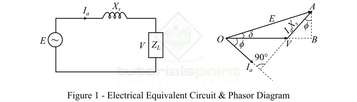
From the phasor diagram, we get,
$$\mathrm{\mathit{AB}\:=\:\mathit{I_{a}X_{s}cos\phi }\:=\:\mathit{E}\:\mathrm{sin\delta }}$$
$$\mathrm{\Rightarrow \mathit{I_{a}cos\phi }\:=\:\frac{\mathit{E\:\mathrm{sin\delta }}}{\mathit{X_{s}}}\cdot \cdot \cdot (2)}$$
Now, from equation (1) & (2), we get,
$$\mathrm{\mathit{P_{0}}\:=\:\frac{3\mathit{EV\:\mathrm{sin\delta }}}{\mathit{X_{s}}}\cdot \cdot \cdot (3)}$$
The expression in Equation-3 gives the approximate output power of a three-phase alternator.
When the alternator is operating at a constant speed with a constant field current, then Xs and E both are constant and therefore the terminal voltage V is also constant. Thus, from Equation-3, we can observe,
$$\mathrm{\mathit{P_{0}}\propto \:\mathrm{sin\delta }}$$
We know, when $\delta$ = 90, then
$$\mathrm{\mathrm{sin\:90^{\circ}}\:=\:1}$$
Thus, the alternator supplies maximum power at $$ =90, and it is given by,
$$\mathrm{\mathit{P_{max}}\:=\:\frac{3\mathit{EV}}{\mathit{X_{s}}}}\cdot \cdot \cdot (4)$$
The maximum power given by Equation-4 is called the static stability limit of the alternator.
Numerical Example
A 3-phase, 11 kV, 3 MVA star-connected alternator has a per phase synchronous reactance of 10 $\Omega$. Its excitation is such that the generated line EMF is 15 kV. When the alternator is connected to infinite busbars. Calculate the maximum output power of the alternator at the given excitation when armature resistance is neglected.
Solution
Given data,
$$\mathrm{\mathrm{Line\:voltage,}\mathit{V_{L}}\:=\:11\:kV\:=\:11000\:V}$$
$$\mathrm{\therefore\:\mathrm{Terminal\:voltage\:per\:phase,}\mathit{V}\:=\:\frac{11000}{\sqrt{3}}\:=\:6350.85\:V}$$
$$\mathrm{\mathrm{Generated\:line\:EMF}\:=\:15\:kV\:=\:15000\:V}$$
$$\mathrm{\therefore\:\mathrm{Generated\:EMF\:per\:phase,}\mathit{E}\:=\:\frac{15000}{\sqrt{3}}\:=\:8660.25\:V}$$
$$\mathrm{\mathrm{Synchronous\: reactance\: per\: phase,}\:\mathit{X_{s}}\:=\:10\:\Omega }$$
Therefore, the maximum power output of the alternator will be,
$$\mathrm{\mathit{P_{max}}\:=\:\frac{3\mathit{EV}}{\mathit{X_{s}}}\:=\:\frac{3\times 8660.25\times 6350.85}{10}}$$
$$\mathrm{\therefore \mathit{P_{max}}\:=\:16499\times 10^{3}W\:=\:16499\:\mathrm{kW}}$$
Losses and Efficiency of 3-Phase Alternator
Losses in Three-Phase Alternator
The losses that occur in a three-phase alternator may be divided into the following four categories −
Copper losses
Iron or core losses
Mechanical losses
Stray load losses
Read through this section to find out more about the types of losses that occur in a three-phase alternator.
Copper Losses
The copper losses occur in the armature winding and rotor winding of the alternator due to their resistance when currents flowing through them. Thus, these losses are also called I2R losses.
Iron or Core Losses
The iron or core losses occur in iron parts like stator core and rotor core of the alternator. These losses consist of hysteresis loss and eddy current loss. The core losses occur because various iron parts of the alternator are subjected to the changing magnetic field.
Mechanical Losses
The mechanical losses occur in the moving or rotating parts like rotor, shaft, bearings, etc. of the alternator. There are two main types of mechanical losses namely, frictional losses and windage losses. The frictional losses are due to friction of bearings in the alternator, while the windage losses are due to friction between the rotating parts of the alternator and the air inside the casing of the alternator.
Stray Load Losses
This category includes those losses in the alternator which cannot be easily determined. These losses are also called miscellaneous losses. The stray load losses may be because of the following reasons −
Distortion of main field flux due to armature reaction.
Non-uniform distribution of current over the area of cross-section of armature conductors.
In practical calculations, we take the stray load losses 1% of the full-load losses.
Note
The iron losses and mechanical losses together are called rotational losses because these losses occur in the alternator due to rotation of the rotor.
All these losses that occur in an alternator are converted into heat and result in the increase of the temperature and decrease in the efficiency of the alternator.
Efficiency of Three-Phase Alternator
The ratio of output power to input power of an alternator is called efficiency of the alternator. The efficiency is usually expressed in percentage.
$\mathrm{\mathrm{Efficiency,} \: \eta \:=\:\frac{Output\:Power}{Input\:Power}\times 100\%\:=\:\frac{Output\:Power}{Output\:Power+Losses}\times 100\%}$
Now, we will derive the expression for efficiency of a three-phase alternator. For that consider a three-phase alternator operating at a lagging power factor.
Let,
V= terminal voltage per phase
Ia = armature current per phase
cos $\phi$ = load power factor (lagging)
Thus, the output power of a three-phase alternator is given by,
$$\mathrm{\mathit{P_{0}}\:=\:3\:\mathit{VI_{a}cos\:\phi }}$$
The losses in the alternator are,
$$\mathrm{\mathrm{Armature\: copper\: loss,}\mathit{P_{cu}}\:=\:3\:\mathit{I_{\mathit{a}}^{\mathrm{2}}R_{a}}}$$
$$\mathrm{\mathrm{Field \:winding\: copper\: loss}\:=\:\mathit{V_{f}I_{f}}}$$
Where,Vf is the DC voltage across field winding and If is the DC field current.
$$\mathrm{\mathrm{Rotational\: losses,}\mathit{P_{r}}\:=\:\mathrm{Core\:losses\:+\:Mechanical\:losses}}$$
$$\mathrm{\mathrm{Stray\:load\:losses}\mathit{P_{s}}}$$
$$\mathrm{\therefore \mathrm{Total\:losses\:in\:alternator,}\mathit{P_{loss}}\:=\:3\:\mathit{I_{a}^{2}R_{a}\:+\:P_{r}\:+\:P_{s}\:+\:V_{f}I_{f}}}$$
Since, the speed of rotation of the rotor is constant so the rotational losses are constant. The field winding copper losses are also constant. If we assume stray-load losses to be constant. Then, we have,
$$\mathrm{\mathrm{Total\:constant\:losses,}\mathit{P_{c}}\:=\:\mathit{P_{r}\:+\:P_{s}\:+\:V_{f}I_{f}}}$$
$$\mathrm{\therefore\:\mathrm{Variable\:losses} \:=\:\mathrm{3}\mathit{I_{a}^{\mathrm{2}}R_{a}}}$$
Hence, the efficiency of the alternator is given by,
$$\mathrm{\eta \:=\:\frac{\mathit{P_{0}}}{\mathit{P_{0}+\mathrm{Losses}}}\:=\:\frac{3\mathit{VI_{a}cos\phi }}{3\mathit{VI_{a}cos\phi \:+\:\mathrm{3}\mathit{I_{a}^{\mathrm{2}}R_{a}}\:+P_{c}}}\cdot \cdot \cdot (1)}$$
Equation-1 can be used to determine the efficiency of a three-phase alternator.
Condition for Maximum Efficiency
The efficiency of an alternator will be maximum when the variable losses are equal to the constant losses, i.e.,
$$\mathrm{\mathit{P_{c}}\:=\:3\:\mathit{I_{a}^{\mathrm{2}}R_{a}}\cdot \cdot \cdot (2)}$$
In practice, the maximum efficiency of an alternator usually occurs at about 85% of the full rated load.
Numerical Example
A three-phase alternator has a per phase terminal voltage of 230 V, and the per phase armature current of 14.4 A. The resistance of the armature circuit of the alternator is 0.5, and the constant losses are 200 watts. Calculate the efficiency and maximum efficiency of the alternator if it is suppling a load at 0.8 lagging power factor.
Solution
$$\mathrm{\mathrm{Efficiency,}\eta \:=\:\frac{3\mathit{VI_{a}cos\phi }}{3\mathit{VI_{a}cos\phi \:+\:\mathrm{3}\mathit{I_{a}^{\mathrm{2}}R_{a}}\:+P_{c}}}}$$
$$\mathrm{\Rightarrow\:\eta \:=\:\frac{3\times 230\times 14.4\times 0.8}{\left ( 3\times 230\times 14.4\times 0.8 \right )\:+\:\left ( 3\times 14.4^{2}\times 0.5 \right )\:+\:200}}$$
$$\mathrm{\therefore \eta \:=\:0.9395\:=\:93.95\%}$$
For maximum efficiency of the alternator,
$$\mathrm{\mathit{P_{c}}\:=\:3\:\mathit{I_{a}^{\mathrm{2}}R_{a}}}$$
$$\mathrm{\therefore \eta_{max} \:=\:\frac{3\mathit{VI_{a}cos\phi }}{3\mathit{VI_{a}cos\phi \:+\:\mathrm{2}\mathit{P_{c}}}}\:=\:\frac{3\times 230\times 14.4\times 0.8}{\left ( 3\times 230\times 14.4\times 0.8 \right )\:+\:\left (2\times 200 \right )}}$$
$$\mathrm{\therefore \eta_{max} \:=\:0.9521\:=\:95.21\%}$$
Working of 3-Phase Synchronous Motor
A three-phase synchronous machine which converts three-phase electrical energy into mechanical energy is called a three-phase synchronous motor.
A three-phase synchronous motor is a constant speed machine, and it runs at the synchronous speed. The synchronous speed of a three-phase synchronous motor is given by,
$$\mathrm{\mathit{N_{s}}\:=\:\frac{120\mathit{f}}{\mathit{p}}\cdot \cdot \cdot (1)}$$
Where,f is the supply frequency andP is the number of field poles in the motor.
Like any other electric motor, a 3-phase synchronous motor also consists of two main parts namely stator and rotor. The stator houses a 3-phase armature winding and receives power from a 3-phase ac supply source. The rotor is a rotating part and carries field winding which is excited from an external source of DC power.
The most important drawback of a synchronous motor is that it is not self-starting and therefore an auxiliary mean has to be used for starting it.
Working of 3-Phase Synchronous Motor
Consider a three-phase synchronous motor having a salient-pole type rotor of two poles namely $\mathit{N_{\mathrm{2}}}$ and $\mathit{S_{\mathrm{2}}}$. Thus, the stator will also be wound for two poles which are $\mathit{N_{\mathrm{1}}}$ and $\mathit{S_{\mathrm{1}}}$. A direct voltage is applied to the rotor winding and a balanced three-phase ac voltage to the stator winding.
The stator winding produces a rotating magnetic field which revolves around the stator at a speed called synchronous speed ($\mathit{N_{\mathit{s}}}$).The direct current flowing through the rotor winding produces two field poles in the rotor and the magnetic field due to these poles is stationary so long as the rotor is not running. Hence, in this case we have a pair of revolving armature poles $\left ( \mathit{N_{\mathrm{1}}}-\mathit{S_{\mathrm{1}}} \right )$ and a pair of stationary rotor poles $\left ( \mathit{N_{\mathrm{2}}}-\mathit{S_{\mathrm{2}}} \right )$.
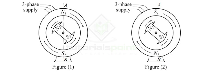
Now, consider an instant at which the stator poles are at positions A and B as shown in Figure-1. It is clear that poles $\mathit{N_{\mathrm{1}}}$ and $\mathit{N_{\mathrm{2}}}$ repel each other and so do the poles $\mathit{S_{\mathrm{1}}}$ and $\mathit{S_{\mathrm{1}}}$. Thus, the rotor tends to rotate in the anticlockwise direction. After a period of half-cycle of AC supply, the polarities of stator poles are reversed, but the polarities of the rotor poles remain the same as shown in Figure-2. In this situation, poles $\mathit{S_{\mathrm{1}}}$ and $\mathit{N_{\mathrm{2}}}$ attract each other and so do the poles $\mathit{N_{\mathrm{1}}}$ and $\mathit{S_{\mathrm{2}}}$. Thus, the rotor now tends to rotate in the clockwise direction.
Since, the stator poles are changing their polarities rapidly, they tend to pull the rotor first in one direction and after half-cycle of ac in the other direction. Because of the bidirectional torque on the rotor and high inertia of the rotor, the synchronous motor fails to start. Therefore, a synchronous motor has no self-starting torque.
Making a Synchronous Motor Self-Starting
A synchronous motor cannot start by itself. To make the motor self-starting, a squirrel-cage winding, called damper winding, is provided on the rotor. The damper winding consists of copper bars embedded in the slots cut on in the pole faces of the salient poles of the rotor, as shown in Figure-3.
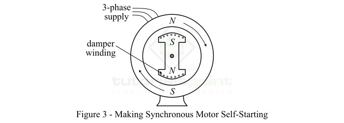
These damper windings serve to start the synchronous motor by itself, which is explained below −
Initially, a 3-phase supply is fed to the stator winding while the rotor winding is left open. The rotating magnetic field of the stator winding induces currents in the damper windings, and due to electromagnetic forces, the rotor starts moving. Thus, the synchronous motor is started as an induction motor.
Once the motor attains a speed nearly equal to the synchronous speed, the rotor winding is excited from a source of dc supply. Now, the resulting poles on the rotor face the stators pole of opposite polarity, and a strong magnetic attraction is set up between them. Thus, the rotor poles are locked with the rotating poles of the stator. Consequently, the rotor revolves at the same speed of the stator poles, i.e. synchronous speed.
Since the rotor is now rotating at the same speed as the stator field, the damper bars do not cut any flux, hence have no induced currents in them. Thus, the damper windings of the rotor are, in effect, removed from the operation of the motor.
In this way, a synchronous motor is made self-starting. It must be noted that due to magnetic interlocking between the stator and rotor poles, the synchronous motor can only run at synchronous speed.
Equivalent Circuit and Power Factor of Synchronous Motor
Equivalent Circuit of Synchronous Motor
A synchronous motor is a doubly excited system which means it is connected to two electrical systems, where a three-phase ac supply is connected to the armature winding and a DC supply to the rotor winding. Figure-1 shows the per phase equivalent circuit of a three-phase synchronous motor.
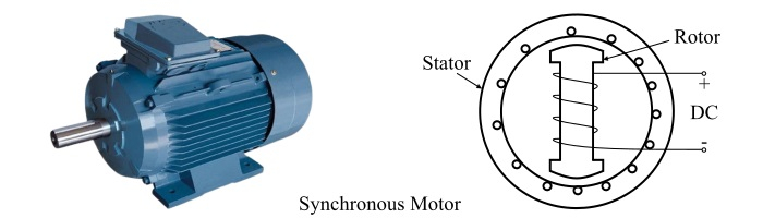
Here,V is the voltage per phase applied to the motor, Rais the armature resistance per phase, and $X_{s}$ is the synchronous reactance per phase. These two parameters (i.e. $R_{a}$ and $X_{s}$) give the synchronous impedance per phase ($Z_{s}$) of the motor.
From the equivalent circuit of the synchronous motor as shown in Figure-1, we can write its voltage equation as,
$$\mathrm{\mathit{V}\:=\:\mathit{E_{b}+I_{a}Z_{s}}}$$
$$\mathrm{\Rightarrow \mathit{V}\:=\:\mathit{E_{b}+I_{a}\left ( R_{a} +jX_{s}\right )}}$$
Where, the bold letters represent the phasor quantities.
Therefore, the armature current per phase is given by
$$\mathrm{I_{a}\:=\:\frac{\mathit{V-E_{b}}}{\mathit{Z_{s}}}\:=\:\frac{\mathit{V-E_{b}}}{\left ( \mathit{R_{a}+jX_{s}}\right )}\:=\:\frac{\mathit{E_{r}}}{\mathit{R_{a}+jX_{s}}}}$$
Where,$\mathit{E_{r}}$ is the resultant voltage in the armature circuit.
The armature current and synchronous impedance of a synchronous motor are the phasor quantities having magnitude and phase angle. Thus, the magnitude of the armature current is given by,
$$\mathrm{\left|I_{a} \right|\:=\:\frac{\mathit{V-E_{b}}}{\mathit{Z_{s}}}\:=\:\frac{\mathit{E_{r}}}{\mathit{Z_{s}}}}$$
And, the magnitude of the synchronous impedance is given by,
$$\mathrm{\left|Z_{s} \right|\:=\:\sqrt{\mathit{R_{a}^{\mathrm{2}}+X_{s}^{\mathrm{2}}}}}$$
The equivalent circuit and the above equations helps a lot in understanding the operation of a synchronous motor as,
When the field excitation is such that $\mathit{E_{b}=V}$, then the synchronous motor is said to be normally excited.
When the field excitation is such that $\mathit{E_{b}<V}$, then the synchronous motor is said to be under excited.
When the field excitation is such that $\mathit{E_{b}> V}$, then the synchronous motor is said to be over excited.
As we shall see in the next section that the excitation of the synchronous motor affects its power factor.
Power Factor of Synchronous Motor
One of the most important characteristics of a synchronous motor is that it can be made to operate at leading, lagging or unity power factor by changing the field excitation. The following discussion explains how the change in field excitation affects the power factor of a synchronous motor −
When the rotor excitation current is such that it produces all the required magnetic flux, then there is no need of extra reactive power in the machine. Consequently, the motor will operate at unity power factor.
When the rotor excitation current is less than that required, i.e., the motor is under-excited. In this case, the motor will draw reactive power from the supply to provide the remaining flux. Thus, the motor will operate at a lagging power factor.
When the rotor excitation current is more than that required, i.e. the motor is over-excited. In this case, the motor will supply reactive power to the 3-phase line, and behaves as a source of reactive power. Consequently, the motor will operate at a leading power factor.
Hence, we may conclude that a synchronous motor absorbs reactive power when it is under-excited and delivers reactive power when it is over-excited.
Power Developed by Synchronous Motor
In this chapter, we will derive the expression for mechanical power developed (Pm) by a three-phase synchronous motor. Here, we will neglect the armature resistance Ra of the synchronous motor. Then, the armature copper loss will be zero and hence the mechanical power developed by the motor is equal to the input power (Pin) to the motor, i.e.,
$$\mathrm{\mathit{P_{m}}\:=\:\mathit{P_{in}}}$$
Now, consider an under-excited (i.e.,Eb<V) three-phase synchronous motor having zero armature resistance (i.e.,Ra = 0), and is driving a mechanical load.
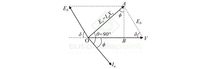
The phasor diagram of one phase of this synchronous motor is shown in the figure. Because the motor is under-excited, thus it will operate at a lagging power factor, say (cos $\phi$). From the phasor diagram, it is clear that $\mathit{E_{r}}\:=\:I_{a}X_{s}$ and the armature current per phase $I_{a}$ lags the resultant EMF $\mathit{E_{r}}$ by an angle of 90.
Therefore, the input power per phase to the motor is given by,
$$\mathrm{\mathit{P_{in}}\:=\mathit{VI_{a}}\:cos\:\phi \:\cdot \cdot \cdot (1)}$$
Since $\mathit{P_{m}}$ is equal to $\mathit{P_{in}}$, therefore,
$$\mathrm{\mathit{P_{m}}\:=\mathit{VI_{a}}\:cos\:\phi \:\cdot \cdot \cdot (2)}$$
From the phasor diagram, we have,
$$\mathrm{\mathit{AB}\:=\mathit{I_{a}X_{s}}\:cos\:\phi \:=\:\mathit{E}_{\mathit{b}}\:sin\:\delta}$$
$$\mathrm{\therefore \mathit{I_{a}\:cos\phi \:=\:\frac{E_{b}\:sin\delta }{\mathit{X_{s}}}}\:\cdot \cdot \cdot (3)}$$
Using equations (2) & (3), we obtain,
$$\mathit{P_{m}\:=\:\frac{\mathit{VE_{b}}sin\delta }{X_{s}}}\cdot \cdot \cdot (4)$$
This is the expression for mechanical power developed (Pm) per phase by the synchronous motor.
For 3-phases of the motor, the developed mechanical power is given by,
$$\mathit{P_{m}\:=\:\frac{3\mathit{VE_{b}}sin\delta }{X_{s}}}\cdot \cdot \cdot (5)$$
Also, from the equations (4) & (5), it is clear that the mechanical power developed will be maximum when power angle ($\delta$= 90) electrical. Therefore,
For per phase,
$$\mathit{P_{max}\:=\:\frac{\mathit{VE_{b}}}{X_{s}}}\cdot \cdot \cdot (6)$$
For 3-phase,
$$\mathit{P_{max}\:=\:\frac{\mathit{3VE_{b}}}{X_{s}}}\cdot \cdot \cdot (7)$$
Important Points
The following important points may be noted about the mechanical power developed by a three-phase synchronous motor −
The mechanical power developed by the synchronous motor increases with the increase in power angle ($\delta$) and vice-versa.
If power angle ($\delta$) is zero, then the synchronous motor cannot develop mechanical power.
When the field excitation of the synchronous motor is reduced to zero, i.e., ($E_{b}$ = 0), the mechanical power developed by the motor is also zero, i.e. the motor will come to a stop.
Numerical Example
A 3-phase, 4000 kW, 3.3 kV, 200 RPM, 50 Hz synchronous motor has per phase synchronous reactance of 1.5 $\Omega$. At full-load, the power angle is 22 electrical. If the generated back EMF per phase is 1.7 kV, calculate the mechanical power developed. What will be the maximum mechanical power developed?
Solution
Given data,
Voltage per phase, $\mathit{V}\:=\:\frac{3.3}{\sqrt{3}}\:=\:1.9\:kV$
Back EMF per phase,$\mathit{E_{b}}\:=\:1.7\:kV$
Synchronous reactance,$X_{s}\:=\:1.5\Omega $
Power angle,$\delta \:=\:22^{^{\circ}}$
Therefore, the mechanical power developed by the motor is,
$$\mathrm{\mathit{P_{m}}\:=\:\frac{3\:\mathit{VE_{b}\:sin\delta} }{\mathit{X_{s}}}\:=\:\frac{3\times 1.9\times 1.7\times \mathrm{sin}\:22^{\circ}}{1.5}}$$
$$\mathit{\therefore P_{m}}\:=\:2.42\times 10^{6}\:W\:=\:2.42\:MW$$
The mechanical power developed will be maximum when ($\delta$ =90),
$$\mathit{P_{max}}\:=\:\frac{3\mathit{VE_{b}}}{X_{s}}\:=\:\frac{3\times 1.9\times 1.7}{1.5}$$
$$\mathit{\therefore P_{max}}\:=\:6.46\:\mathrm{MW}$$
