
Article Categories
- All Categories
-
 Data Structure
-
 Networking
-
 RDBMS
RDBMS
-
 Operating System
-
 Java
Java
-
 MS Excel
-
 iOS
iOS
-
 HTML
HTML
-
 CSS
CSS
-
 Android
-
 Python
-
 C Programming
-
 C++
C++
-
 C#
C#
-
 MongoDB
-
 MySQL
MySQL
-
 Javascript
-
 PHP
PHP
-
 Economics & Finance
Visual representations of Outputs/Activations of each CNN layer
Introduction
Convolutional neural networks offer remarkable insight into mimicking human?like visual processing through their sophisticated multi?layer architectures. This article has taken you on a creative journey through each layer's function and provided visual representations of their outputs or activations along the way. As researchers continue to unlock even deeper levels of understanding within CNNs, we move closer toward unraveling the mysteries behind complex intelligence exhibited by these futuristic machines. In this article, we embark on a fascinating journey through the layers of CNNs to unravel how these remarkable machines work.
Visual representation of Outputs
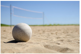
The Input Layer ? Where It All BeginsThe input layer receives visual information in its raw form, such as an image or video frame with pixel values encoding color and texture details. This layer acts as a canvas upon which subsequent layers paint increasingly abstract representations
Convolutional Layers ? From Basic Shapes to Complex Features
-
In these early stages lies a set of convolutional layers responsible for feature detection at different scales and orientations. They achieve this by applying small filters over local regions of the input images, learning distinctive patterns like edges or textures automatically.
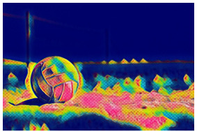
Visual Representation: Imagine observing activations from one such filter designed to detect diagonal edges; we might see areas with high activation corresponding to different angles on diagonal lines across diverse parts of our original image.
-
Activation Functions ? Infusing Non?Linearity
After every convolution operation within each layer comes an activation function (e.g., ReLU). These functions inject non?linear behavior into CNNs, allowing them to model intricate relationships among detected features effectively.
Visual Representation: Examining activated pixels after applying ReLU activation illuminates what parts of our feature maps are actively contributing valuable information based on changes reflected across before?and?after comparisons
-
Pooling Layers ? Downsampling While Preserving Essential Details
Pooling operations reduce spatial dimensions while retaining key information learned during previous convolutions. Popular pooling techniques include max?pooling, which retains the highest activations within a local neighborhood, and average?pooling.
Visual Representation: Visualizing outputs of pooled regions demonstrates their ability to focus on vital features independently of exact pixel positions or irrelevant background noise.
-
Fully Connected Layers ? Understanding Higher?Level Concepts
These layers integrate extracted features from previous convolutional stages into higher?level representations and enable comprehensive classifications or predictions.
Visual Representation: By inspecting activations in these densely connected layers, we can gain insights into how specific objects or concepts are encoded as patterns across multiple feature maps contributing to the final output prediction.
Grad?CAM method
The Grad?CAM technique aims to find important regions by using gradient information within a given CNN layer. In CNN layer, the input image is first given and it contributes most to certain class predictions, later offers more localized visualizations.
Algorithm
Step 1 :The Grad?CAM algorithm is implemented in Python using the Keras and vis packages.
Step 2 :The target class index is set and a pre?trained ResNet50 model with weights from the ImageNet dataset is loaded.
Step 3 :The Grad?CAM technique is then used to create a heatmap visualization for the desired class index, which is then superimposed on the original picture.
Step 4 :The last image is the overlay one, is displayed.
Example
#importing the required modules
from keras.applications.resnet50 import ResNet50, preprocess_input, decode_predictions
from vis.visualization import visualize_cam

# Loading the pre-trained ResNet50 model with weights trained on ImageNet dataset.
model = ResNet50(weights='imagenet')

# Defining target class index (e.g., 630 corresponds to "Donut" class).
class_index = 630

cam_map = visualize_cam(model=model,
                        layer_idx=-1,
                        filter_indices=class_index,
                        seed_input=img,
                        penultimate_layer_idx=get_penultimate_layer_id(model))

heat_map = np.uint8(cm.jet(cam_map)[..., :3] * 255)
superimposed_img=overlay(cam_img_path='path_to_original_image',
                           cam_heatmap=heat_map)

plt.imshow(superimposed_img)
Input image needs to be saved in local machine and the path can be given in code
Output image of Heat Map visualization
Conclusion
The Activation Maximization (AM) technique aims to find an image that maximizes a specific neuron's activation within a given CNN layer. By optimizing this objective function iteratively using gradient ascent methods, we can generate highly informative images that activate neurons strongly. The multi?layer architecture of CNNs, where each layer extracts progressively complicated features from raw input data, is a key factor in their effectiveness.
348 Views
