Top 10 Machine Learning Algorithms For Beginners

Introduction

The definition of manual is evolving in a world when almost all manual operations are mechanized. There are many different kinds of machine learning algorithms available today, some of which can help computers learn, get smarter, and resemble humans more. Because technology is advancing rapidly right now, it is possible to anticipate the future by looking at how computers have changed over time.

Many different machine learning algorithms have been developed in these extremely dynamic times to aid in resolving difficult real-world problems. The automated, selfcorrecting ML algorithms will get better over time. Let's look at the various sorts of machine learning algorithms and how they are categorised before addressing the top 10 machine learning algorithms everyone should be familiar with.

Machine learning algorithms are classified into 4 types −

• Supervised

• Unsupervised Learning

• Semi-supervised Learning

• Reinforcement Learning

These four ML algorithm types are divided into further categories.

Top 10 Machine Learning Algorithms For Beginners

• Linear Regression

• Logistic regression

• Decision Trees

• KNN Classification

• Recurrent Neural Networks (RNN)

• Support Vector Machine (SVM)

• Random Forest

• K-means Clustering

• Naive Bayes theorem

• Artificial Neural Network

1. Linear Regression

The machine learning community adopted it to create predictions based on the linear regression equation after it was first developed in statistics to investigate the relationship between input and numerical variables.

The mathematical definition of linear regression is a linear equation that combines a specific set of input data (x) to predict the output value (y) for that set of input values. Each set of input values is given a factor by the linear equation. These factors are known as the coefficients and are denoted by the Greek letter Beta ().

A linear regression model with two sets of input values, x1 and x2, is represented by the equation below. The coefficients of the linear equation are 0, 1, and 2, and y represents the output of the model.

y = β0 + β1x1 + β2x2

The linear equation depicts a straight line when there is just one input variable. For the sake of simplicity, let's assume that x2 has no impact on the results of the linear regression model and that 2 is equal to zero. The linear regression in this situation will seem as a straight line, and its equation is provided below.

y = β0 + β1x1

Below is a graph of the linear regression equation model.

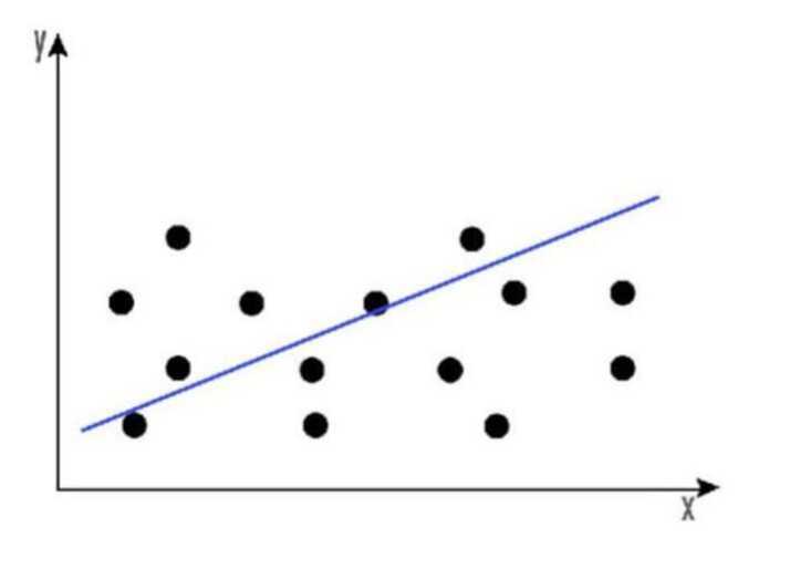
The overall price trend of a stock over time can be discovered using linear regression. This aids in determining if the price change keeps rising or negative.

2. Logistic Regression

Logistic regression is used to estimate discrete values (typically binary values like 0/1) from a set of independent variables. It helps predict the likelihood of an event by converting the data to a logit function. sometimes referred to as logit regression.

The techniques described below are frequently employed to enhance logistic regression models −

• put interaction phrases in

• remove components.

• A non-linear model is used

• regularizing methods.

The following equation yields the sigmoid/logistic function.

y = 1 / (1+ e-x)

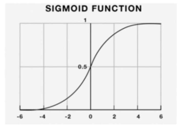
Logistic regression can be used to anticipate the market's direction, to put it simply.

3. Decision Tress

Decision trees are essentially a support tool that resembles a tree and can be used to depict a cause and its impact. It can effectively classify both discrete and continuous dependent variables. This method divides the population into two or more homogeneous sets based on the most significant traits or independent variables.

Decision trees have the drawback of being prone to overfitting because of their inherent structural system.

4. KNN Classification

Problems involving classification and regression can both be solved using this approach. It appears that the solution of categorization issues is more frequently applied within the Data Science business. It is a straightforward algorithm that sorts new instances by getting the consent of at least k of its neighbours and then saves all of the existing cases. The case is then given to the class that it most closely resembles. A distance function is used to calculate this.

KNN is simple to comprehend when compared to reality. For instance, it makes perfect sense to speak with a person's friends and coworkers if we want to learn more about them.

Consider the following factors before using the K Nearest Neighbors algorithm −

• To avoid algorithm partiality, higher range variables should be normalised.

• Data preprocessing is still required.

• KNN has a significant computational cost.

5. Recurrent Neural Networks (RNN)

The processing of sequential data, where each data unit depends on the one before it, is made simple by RNNs, a particular type of neural network that contains a memory attached to each node. The benefit of RNN over a typical neural network can be explained by the fact that a word is expected to be processed character by character. By the time it reached the letter "d," a node in a standard neural network would have forgotten the letter "t" in the word "trade," but a node in a recurrent neural network will remember the letter since it has its own memory.

6. Support Vector Machine (SVM)

Data can be classified using the SVM method by presenting the raw data as dots in an ndimensional space (where n is the number of features you have). The data can then be easily categorised after each feature's value is connected to a specific coordinate. Classifier lines can be used to separate the data into groups and plot them on a graph.

A hyperplane that serves as a division between the categories is produced by the SVM algorithm. A new data point is evaluated by the SVM algorithm and is categorised according to which side it appears on.

7. Random Forest

To address some of the drawbacks of decision trees, a random forest algorithm was created.

Decision trees, that are graphs of decisions expressing their action course or statistical probability, are part of the Random Forest. These several trees are used to form the Classification and Regression (CART) Model, which is a single tree. Each tree assigns a classification that is referred to as a "vote" for that class in order to categorise an item based on its qualities. The classification with the most votes is then selected by the forest. Regression takes into account the average of the results from various trees.

According to the following, Random Forest operates −

• Assume there are N cases total. The training set is chosen as a subset of these N examples.

• Assuming that there are M input variables, m is chosen so that m M. The node is divided using the optimal split between m and M. The amount of m is maintained constant as the trees enlarge.

• The size of each tree is maximized.

• Predict the new data by combining the predictions of n trees (i.e., majority votes for classification, average for regression).

8. K-means Clustering

It is an unsupervised learning method that deals with clustering problems. The division of data sets into a predetermined number of clusters, let's say K, ensures that the data points within each cluster are homogeneous and separate from those within the other clusters.

9. Naive Bayes theorem

The core element of a Naive Bayes classifier is that the presence of one feature in a class has no bearing on the presence of any other characteristics.

A Naive Bayes classifier would take into account each of these attributes separately when determining the probability of a specific outcome, even if these characteristics are related to one another. A Naive Bayesian model is effective and simple to construct for large datasets. Despite being simple, it has been shown to outperform even the most sophisticated categorization methods.

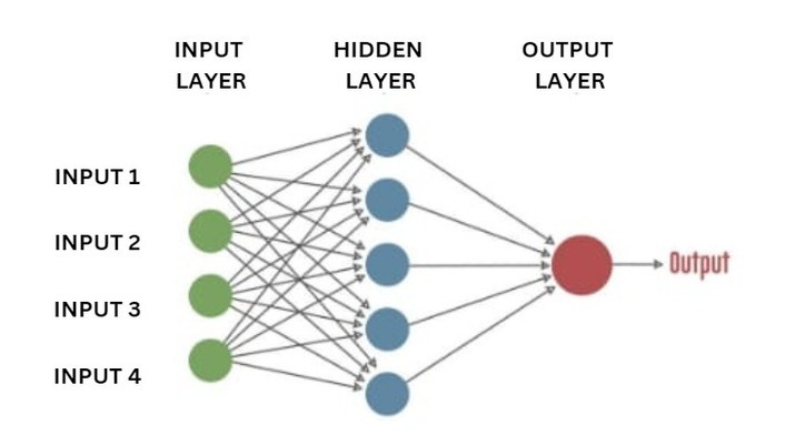
10. Artificial Neural Network

One of our greatest accomplishments is an artificial neural network. As seen in the illustration, we have established a number of nodes that are connected to one another to represent the neurons in our brain. Simply explained, each neuron receives information from another neuron, processes it, and then sends the results to the other neuron as an output.

An artificial neuron is represented by each circular node, and a link between one neuron's output and another's input is represented by an arrow.

Conclusion

The ten machine algorithms that any data scientist has to be familiar with are listed above. The selection of which data science algorithm to utilise is a very common one made by beginners to the field. The right decision for this component depends totally on a few key factors, such as the size, the quality level, the type of data, the available processing time, job priorities, and the intended use of the data.

In order to achieve the best results, pick any one of the algorithms listed above, regardless of the level of competence in the field of data science.