- Keras - Home
- Keras - Introduction
- Keras - Installation
- Keras - Backend Configuration
- Keras - Overview of Deep learning
- Keras - Deep learning
- Keras - Modules
- Keras - Layers
- Keras - Customized Layer
- Keras - Models
- Keras - Model Compilation
- Keras - Model Evaluation and Prediction
- Keras - Convolution Neural Network
- Keras - Regression Prediction using MPL
- Keras - Time Series Prediction using LSTM RNN
- Keras - Applications
- Keras - Real Time Prediction using ResNet Model
- Keras - Pre-Trained Models
- Keras Useful Resources
- Keras - Quick Guide
- Keras - Useful Resources
- Keras - Discussion
Keras - Regression Prediction using MPL
In this chapter, let us write a simple MPL based ANN to do regression prediction. Till now, we have only done the classification based prediction. Now, we will try to predict the next possible value by analyzing the previous (continuous) values and its influencing factors.
The Regression MPL can be represented as below −
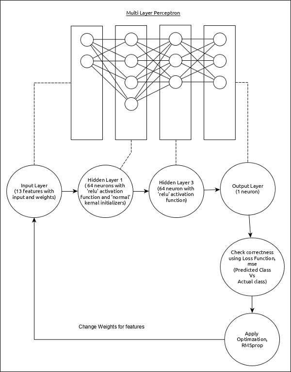
The core features of the model are as follows −
Input layer consists of (13,) values.
First layer, Dense consists of 64 units and relu activation function with normal kernel initializer.
Second layer, Dense consists of 64 units and relu activation function.
Output layer, Dense consists of 1 unit.
Use mse as loss function.
Use RMSprop as Optimizer.
Use accuracy as metrics.
Use 128 as batch size.
Use 500 as epochs.
Step 1 − Import the modules
Let us import the necessary modules.
import keras

from keras.datasets import boston_housing
from keras.models import Sequential
from keras.layers import Dense
from keras.optimizers import RMSprop
from keras.callbacks import EarlyStopping
from sklearn import preprocessing
from sklearn.preprocessing import scale
Step 2 − Load data
Let us import the Boston housing dataset.
(x_train, y_train), (x_test, y_test) = boston_housing.load_data()
Here,
boston_housing is a dataset provided by Keras. It represents a collection of housing information in Boston area, each having 13 features.
Step 3 − Process the data
Let us change the dataset according to our model, so that, we can feed into our model. The data can be changed using below code −
x_train_scaled = preprocessing.scale(x_train)
scaler = preprocessing.StandardScaler().fit(x_train)
x_test_scaled = scaler.transform(x_test)
Here, we have normalized the training data using sklearn.preprocessing.scale function. preprocessing.StandardScaler().fit function returns a scalar with the normalized mean and standard deviation of the training data, which we can apply to the test data using scalar.transform function. This will normalize the test data as well with the same setting as that of training data.
Step 4 − Create the model
Let us create the actual model.
model = Sequential()
model.add(Dense(64, kernel_initializer = 'normal', activation = 'relu',
input_shape = (13,)))
model.add(Dense(64, activation = 'relu')) model.add(Dense(1))
Step 5 − Compile the model
Let us compile the model using selected loss function, optimizer and metrics.
model.compile(
   loss = 'mse',
   optimizer = RMSprop(),
   metrics = ['mean_absolute_error']
)
Step 6 − Train the model
Let us train the model using fit() method.
history = model.fit(
   x_train_scaled, y_train,
   batch_size=128,
   epochs = 500,
   verbose = 1,
   validation_split = 0.2,
   callbacks = [EarlyStopping(monitor = 'val_loss', patience = 20)]
)
Here, we have used callback function, EarlyStopping. The purpose of this callback is to monitor the loss value during each epoch and compare it with previous epoch loss value to find the improvement in the training. If there is no improvement for the patience times, then the whole process will be stopped.
Executing the application will give the below information as output −
Train on 323 samples, validate on 81 samples Epoch 1/500 2019-09-24 01:07:03.889046: I
tensorflow/core/platform/cpu_feature_guard.cc:142]
Your CPU supports instructions that this
TensorFlow binary was not co mpiled to use: AVX2 323/323
[==============================] - 0s 515us/step - loss: 562.3129
- mean_absolute_error: 21.8575 - val_loss: 621.6523 - val_mean_absolute_erro
r: 23.1730 Epoch 2/500
323/323 [==============================] - 0s 11us/step - loss: 545.1666
- mean_absolute_error: 21.4887 - val_loss: 605.1341 - val_mean_absolute_error
: 22.8293 Epoch 3/500
323/323 [==============================] - 0s 12us/step - loss: 528.9944
- mean_absolute_error: 21.1328 - val_loss: 588.6594 - val_mean_absolute_error
: 22.4799 Epoch 4/500
323/323 [==============================] - 0s 12us/step - loss: 512.2739
- mean_absolute_error: 20.7658 - val_loss: 570.3772 - val_mean_absolute_error
: 22.0853 Epoch 5/500
323/323 [==============================] - 0s 9us/step - loss: 493.9775
- mean_absolute_error: 20.3506 - val_loss: 550.9548 - val_mean_absolute_error: 21.6547
..........
..........
..........
Epoch 143/500
323/323 [==============================] - 0s 15us/step - loss: 8.1004
- mean_absolute_error: 2.0002 - val_loss: 14.6286 - val_mean_absolute_error:
2. 5904 Epoch 144/500
323/323 [==============================] - 0s 19us/step - loss: 8.0300
- mean_absolute_error: 1.9683 - val_loss: 14.5949 - val_mean_absolute_error:
2. 5843 Epoch 145/500
323/323 [==============================] - 0s 12us/step - loss: 7.8704
- mean_absolute_error: 1.9313 - val_loss: 14.3770 - val_mean_absolute_error: 2. 4996
Step 7 − Evaluate the model
Let us evaluate the model using test data.
score = model.evaluate(x_test_scaled, y_test, verbose = 0)
print('Test loss:', score[0])
print('Test accuracy:', score[1])
Executing the above code will output the below information −
Test loss: 21.928471583946077 Test accuracy: 2.9599233234629914
Step 8 − Predict
Finally, predict using test data as below −
prediction = model.predict(x_test_scaled)
print(prediction.flatten())
print(y_test)
The output of the above application is as follows −
[ 7.5612316 17.583357 21.09344 31.859276 25.055613 18.673872 26.600405 22.403967 19.060272 22.264952
17.4191 17.00466 15.58924 41.624374 20.220217 18.985565 26.419338 19.837091 19.946192 36.43445
12.278508 16.330965 20.701359 14.345301 21.741161 25.050423 31.046402 27.738455 9.959419 20.93039
20.069063 14.518344 33.20235 24.735163 18.7274 9.148898 15.781284 18.556862 18.692865 26.045074
27.954073 28.106823 15.272034 40.879818 29.33896 23.714525 26.427515 16.483374 22.518442 22.425386
33.94826 18.831465 13.2501955 15.537227 34.639984 27.468002 13.474407 48.134598 34.39617
22.8503124.042334 17.747198 14.7837715 18.187277 23.655672 22.364983 13.858193 22.710032 14.371148
7.1272087 35.960033 28.247292 25.3014 14.477208 25.306196 17.891165 20.193708 23.585173 34.690193
12.200583 20.102983 38.45882 14.741723 14.408362 17.67158 18.418497 21.151712 21.157492 22.693687
29.809034 19.366991 20.072294 25.880817 40.814568 34.64087 19.43741 36.2591 50.73806 26.968863 43.91787
32.54908 20.248306 ] [ 7.2 18.8 19. 27. 22.2 24.5 31.2 22.9 20.5 23.2 18.6 14.5 17.8 50. 20.8 24.3 24.2
19.8 19.1 22.7 12. 10.2 20. 18.5 20.9 23. 27.5 30.1 9.5 22. 21.2 14.1 33.1 23.4 20.1 7.4 15.4 23.8 20.1
24.5 33. 28.4 14.1 46.7 32.5 29.6 28.4 19.8 20.2 25. 35.4 20.3 9.7 14.5 34.9 26.6 7.2 50. 32.4 21.6 29.8
13.1 27.5 21.2 23.1 21.9 13. 23.2 8.1 5.6 21.7 29.6 19.6 7. 26.4 18.9 20.9 28.1 35.4 10.2 24.3 43.1 17.6
15.4 16.2 27.1 21.4 21.5 22.4 25. 16.6 18.6 22. 42.8 35.1 21.5 36. 21.9 24.1 50. 26.7 25. ]
The output of both array have around 10-30% difference and it indicate our model predicts with reasonable range.
