- Keras - Home
- Keras - Introduction
- Keras - Installation
- Keras - Backend Configuration
- Keras - Overview of Deep learning
- Keras - Deep learning
- Keras - Modules
- Keras - Layers
- Keras - Customized Layer
- Keras - Models
- Keras - Model Compilation
- Keras - Model Evaluation and Prediction
- Keras - Convolution Neural Network
- Keras - Regression Prediction using MPL
- Keras - Time Series Prediction using LSTM RNN
- Keras - Applications
- Keras - Real Time Prediction using ResNet Model
- Keras - Pre-Trained Models
- Keras Useful Resources
- Keras - Quick Guide
- Keras - Useful Resources
- Keras - Discussion
Keras - Convolution Neural Network
Let us modify the model from MPL to Convolution Neural Network (CNN) for our earlier digit identification problem.
CNN can be represented as below −
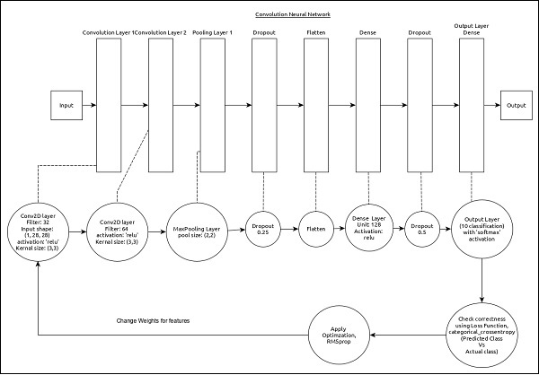
The core features of the model are as follows −
Input layer consists of (1, 8, 28) values.
First layer, Conv2D consists of 32 filters and relu activation function with kernel size, (3,3).
Second layer, Conv2D consists of 64 filters and relu activation function with kernel size, (3,3).
Thrid layer, MaxPooling has pool size of (2, 2).
Fifth layer, Flatten is used to flatten all its input into single dimension.
Sixth layer, Dense consists of 128 neurons and relu activation function.
Seventh layer, Dropout has 0.5 as its value.
Eighth and final layer consists of 10 neurons and softmax activation function.
Use categorical_crossentropy as loss function.
Use Adadelta() as Optimizer.
Use accuracy as metrics.
Use 128 as batch size.
Use 20 as epochs.
Step 1 − Import the modules
Let us import the necessary modules.
import keras
from keras.datasets import mnist
from keras.models import Sequential
from keras.layers import Dense, Dropout, Flatten
from keras.layers import Conv2D, MaxPooling2D
from keras import backend as K
import numpy as np
Step 2 − Load data
Let us import the mnist dataset.
(x_train, y_train), (x_test, y_test) = mnist.load_data()
Step 3 − Process the data
Let us change the dataset according to our model, so that it can be feed into our model.
img_rows, img_cols = 28, 28

if K.image_data_format() == 'channels_first':
   x_train = x_train.reshape(x_train.shape[0], 1, img_rows, img_cols)
   x_test = x_test.reshape(x_test.shape[0], 1, img_rows, img_cols)
   input_shape = (1, img_rows, img_cols)
else:
   x_train = x_train.reshape(x_train.shape[0], img_rows, img_cols, 1)
   x_test = x_test.reshape(x_test.shape[0], img_rows, img_cols, 1)
   input_shape = (img_rows, img_cols, 1)

x_train = x_train.astype('float32')
x_test = x_test.astype('float32')
x_train /= 255
x_test /= 255

y_train = keras.utils.to_categorical(y_train, 10)
y_test = keras.utils.to_categorical(y_test, 10)
The data processing is similar to MPL model except the shape of the input data and image format configuration.
Step 4 − Create the model
Let us create tha actual model.
model = Sequential()
model.add(Conv2D(32, kernel_size = (3, 3),
   activation = 'relu', input_shape = input_shape))
model.add(Conv2D(64, (3, 3), activation = 'relu'))
model.add(MaxPooling2D(pool_size = (2, 2)))
model.add(Dropout(0.25)) model.add(Flatten())
model.add(Dense(128, activation = 'relu'))
model.add(Dropout(0.5))
model.add(Dense(10, activation = 'softmax'))
Step 5 − Compile the model
Let us compile the model using selected loss function, optimizer and metrics.
model.compile(loss = keras.losses.categorical_crossentropy,
   optimizer = keras.optimizers.Adadelta(), metrics = ['accuracy'])
Step 6 − Train the model
Let us train the model using fit() method.
model.fit(
   x_train, y_train,
   batch_size = 128,
   epochs = 12,
   verbose = 1,
   validation_data = (x_test, y_test)
)
Executing the application will output the below information −
Train on 60000 samples, validate on 10000 samples Epoch 1/12
60000/60000 [==============================] - 84s 1ms/step - loss: 0.2687
- acc: 0.9173 - val_loss: 0.0549 - val_acc: 0.9827 Epoch 2/12
60000/60000 [==============================] - 86s 1ms/step - loss: 0.0899
- acc: 0.9737 - val_loss: 0.0452 - val_acc: 0.9845 Epoch 3/12
60000/60000 [==============================] - 83s 1ms/step - loss: 0.0666
- acc: 0.9804 - val_loss: 0.0362 - val_acc: 0.9879 Epoch 4/12
60000/60000 [==============================] - 81s 1ms/step - loss: 0.0564
- acc: 0.9830 - val_loss: 0.0336 - val_acc: 0.9890 Epoch 5/12
60000/60000 [==============================] - 86s 1ms/step - loss: 0.0472
- acc: 0.9861 - val_loss: 0.0312 - val_acc: 0.9901 Epoch 6/12
60000/60000 [==============================] - 83s 1ms/step - loss: 0.0414
- acc: 0.9877 - val_loss: 0.0306 - val_acc: 0.9902 Epoch 7/12
60000/60000 [==============================] - 89s 1ms/step - loss: 0.0375
-acc: 0.9883 - val_loss: 0.0281 - val_acc: 0.9906 Epoch 8/12
60000/60000 [==============================] - 91s 2ms/step - loss: 0.0339
- acc: 0.9893 - val_loss: 0.0280 - val_acc: 0.9912 Epoch 9/12
60000/60000 [==============================] - 89s 1ms/step - loss: 0.0325
- acc: 0.9901 - val_loss: 0.0260 - val_acc: 0.9909 Epoch 10/12
60000/60000 [==============================] - 89s 1ms/step - loss: 0.0284
- acc: 0.9910 - val_loss: 0.0250 - val_acc: 0.9919 Epoch 11/12
60000/60000 [==============================] - 86s 1ms/step - loss: 0.0287
- acc: 0.9907 - val_loss: 0.0264 - val_acc: 0.9916 Epoch 12/12
60000/60000 [==============================] - 86s 1ms/step - loss: 0.0265
- acc: 0.9920 - val_loss: 0.0249 - val_acc: 0.9922
Step 7 − Evaluate the model
Let us evaluate the model using test data.
score = model.evaluate(x_test, y_test, verbose = 0)

print('Test loss:', score[0])
print('Test accuracy:', score[1])
Executing the above code will output the below information −
Test loss: 0.024936060590433316
Test accuracy: 0.9922
The test accuracy is 99.22%. We have created a best model to identify the handwriting digits.
Step 8 − Predict
Finally, predict the digit from images as below −
pred = model.predict(x_test)
pred = np.argmax(pred, axis = 1)[:5]
label = np.argmax(y_test,axis = 1)[:5]

print(pred)
print(label)
The output of the above application is as follows −
[7 2 1 0 4]
[7 2 1 0 4]
The output of both array is identical and it indicate our model correctly predicts the first five images.
