Keras - Model Compilation

---

---

Previously, we studied the basics of how to create model using Sequential and Functional API. This chapter explains about how to compile the model. The compilation is the final step in creating a model. Once the compilation is done, we can move on to training phase.

Let us learn few concepts required to better understand the compilation process.

Loss

In machine learning, Loss function is used to find error or deviation in the learning process. Keras requires loss function during model compilation process.

Keras provides quite a few loss function in the losses module and they are as follows −

• mean_squared_error
• mean_absolute_error
• mean_absolute_percentage_error
• mean_squared_logarithmic_error
• squared_hinge
• hinge
• categorical_hinge
• logcosh
• huber_loss
• categorical_crossentropy
• sparse_categorical_crossentropy
• binary_crossentropy
• kullback_leibler_divergence
• poisson
• cosine_proximity
• is_categorical_crossentropy

All above loss function accepts two arguments −

• y_true − true labels as tensors

• y_pred − prediction with same shape as y_true

Import the losses module before using loss function as specified below −

from keras import losses

Optimizer

In machine learning, Optimization is an important process which optimize the input weights by comparing the prediction and the loss function. Keras provides quite a few optimizer as a module, optimizers and they are as follows:

SGD − Stochastic gradient descent optimizer.

keras.optimizers.SGD(learning_rate = 0.01, momentum = 0.0, nesterov = False)

RMSprop − RMSProp optimizer.

keras.optimizers.RMSprop(learning_rate = 0.001, rho = 0.9)

Adagrad − Adagrad optimizer.

keras.optimizers.Adagrad(learning_rate = 0.01)

Adadelta − Adadelta optimizer.

keras.optimizers.Adadelta(learning_rate = 1.0, rho = 0.95)

Adam − Adam optimizer.

keras.optimizers.Adam(
   learning_rate = 0.001, beta_1 = 0.9, beta_2 = 0.999, amsgrad = False
)

Adamax − Adamax optimizer from Adam.

keras.optimizers.Adamax(learning_rate = 0.002, beta_1 = 0.9, beta_2 = 0.999)

Nadam − Nesterov Adam optimizer.

keras.optimizers.Nadam(learning_rate = 0.002, beta_1 = 0.9, beta_2 = 0.999)

Import the optimizers module before using optimizers as specified below −

from keras import optimizers

Metrics

In machine learning, Metrics is used to evaluate the performance of your model. It is similar to loss function, but not used in training process. Keras provides quite a few metrics as a module, metrics and they are as follows

• accuracy
• binary_accuracy
• categorical_accuracy
• sparse_categorical_accuracy
• top_k_categorical_accuracy
• sparse_top_k_categorical_accuracy
• cosine_proximity
• clone_metric

Similar to loss function, metrics also accepts below two arguments −

• y_true − true labels as tensors

• y_pred − prediction with same shape as y_true

Import the metrics module before using metrics as specified below −

from keras import metrics

Compile the model

Keras model provides a method, compile() to compile the model. The argument and default value of the compile() method is as follows

compile(
   optimizer, 
   loss = None, 
   metrics = None, 
   loss_weights = None, 
   sample_weight_mode = None, 
   weighted_metrics = None, 
   target_tensors = None
)

The important arguments are as follows −

• loss function
• Optimizer
• metrics

A sample code to compile the mode is as follows −

from keras import losses 
from keras import optimizers 
from keras import metrics 

model.compile(loss = 'mean_squared_error',  
   optimizer = 'sgd', metrics = [metrics.categorical_accuracy])

where,

• loss function is set as mean_squared_error

• optimizer is set as sgd

• metrics is set as metrics.categorical_accuracy

Model Training

Models are trained by NumPy arrays using fit(). The main purpose of this fit function is used to evaluate your model on training. This can be also used for graphing model performance. It has the following syntax −

model.fit(X, y, epochs = , batch_size = )

Here,

• X, y − It is a tuple to evaluate your data.

• epochs − no of times the model is needed to be evaluated during training.

• batch_size − training instances.

Let us take a simple example of numpy random data to use this concept.

Create data

Let us create a random data using numpy for x and y with the help of below mentioned command −

import numpy as np 

x_train = np.random.random((100,4,8)) 
y_train = np.random.random((100,10))

Now, create random validation data,

x_val = np.random.random((100,4,8)) 
y_val = np.random.random((100,10))

Create model

Let us create simple sequential model −

from keras.models import Sequential model = Sequential()

Add layers

Create layers to add model −

from keras.layers import LSTM, Dense 

# add a sequence of vectors of dimension 16 
model.add(LSTM(16, return_sequences = True)) 
model.add(Dense(10, activation = 'softmax'))

compile model

Now model is defined. You can compile using the below command −

model.compile(
   loss = 'categorical_crossentropy', optimizer = 'sgd', metrics = ['accuracy']
)

Apply fit()

Now we apply fit() function to train our data −

model.fit(x_train, y_train, batch_size = 32, epochs = 5, validation_data = (x_val, y_val))

Create a Multi-Layer Perceptron ANN

We have learned to create, compile and train the Keras models.

Let us apply our learning and create a simple MPL based ANN.

Dataset module

Before creating a model, we need to choose a problem, need to collect the required data and convert the data to NumPy array. Once data is collected, we can prepare the model and train it by using the collected data. Data collection is one of the most difficult phase of machine learning. Keras provides a special module, datasets to download the online machine learning data for training purposes. It fetches the data from online server, process the data and return the data as training and test set. Let us check the data provided by Keras dataset module. The data available in the module are as follows,

• CIFAR10 small image classification
• CIFAR100 small image classification
• IMDB Movie reviews sentiment classification
• Reuters newswire topics classification
• MNIST database of handwritten digits
• Fashion-MNIST database of fashion articles
• Boston housing price regression dataset

Let us use the MNIST database of handwritten digits (or minst) as our input. minst is a collection of 60,000, 28x28 grayscale images. It contains 10 digits. It also contains 10,000 test images.

Below code can be used to load the dataset −

from keras.datasets import mnist 

(x_train, y_train), (x_test, y_test) = mnist.load_data()

where

• Line 1 imports minst from the keras dataset module.

• Line 3 calls the load_data function, which will fetch the data from online server and return the data as 2 tuples, First tuple, (x_train, y_train) represent the training data with shape, (number_sample, 28, 28) and its digit label with shape, (number_samples, ). Second tuple, (x_test, y_test) represent test data with same shape.

Other dataset can also be fetched using similar API and every API returns similar data as well except the shape of the data. The shape of the data depends on the type of data.

Create a model

Let us choose a simple multi-layer perceptron (MLP) as represented below and try to create the model using Keras.

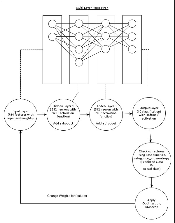
The core features of the model are as follows −

• Input layer consists of 784 values (28 x 28 = 784).

• First hidden layer, Dense consists of 512 neurons and ‘relu’ activation function.

• Second hidden layer, Dropout has 0.2 as its value.

• Third hidden layer, again Dense consists of 512 neurons and ‘relu’ activation function.

• Fourth hidden layer, Dropout has 0.2 as its value.

• Fifth and final layer consists of 10 neurons and ‘softmax’ activation function.

• Use categorical_crossentropy as loss function.

• Use RMSprop() as Optimizer.

• Use accuracy as metrics.

• Use 128 as batch size.

• Use 20 as epochs.

Step 1 − Import the modules

Let us import the necessary modules.

import keras 
from keras.datasets import mnist 
from keras.models import Sequential 
from keras.layers import Dense, Dropout 
from keras.optimizers import RMSprop 
import numpy as np

Step 2 − Load data

Let us import the mnist dataset.

(x_train, y_train), (x_test, y_test) = mnist.load_data()

Step 3 − Process the data

Let us change the dataset according to our model, so that it can be feed into our model.

x_train = x_train.reshape(60000, 784) 
x_test = x_test.reshape(10000, 784) 
x_train = x_train.astype('float32') 
x_test = x_test.astype('float32') 
x_train /= 255 
x_test /= 255 

y_train = keras.utils.to_categorical(y_train, 10) 
y_test = keras.utils.to_categorical(y_test, 10)

Where

• reshape is used to reshape the input from (28, 28) tuple to (784, )

• to_categorical is used to convert vector to binary matrix

Step 4 − Create the model

Let us create the actual model.

model = Sequential() 
model.add(Dense(512, activation = 'relu', input_shape = (784,))) 
model.add(Dropout(0.2)) 
model.add(Dense(512, activation = 'relu'))
model.add(Dropout(0.2)) 
model.add(Dense(10, activation = 'softmax'))

Step 5 − Compile the model

Let us compile the model using selected loss function, optimizer and metrics.

model.compile(loss = 'categorical_crossentropy',     
   optimizer = RMSprop(), 
   metrics = ['accuracy'])

Step 6 − Train the model

Let us train the model using fit() method.

history = model.fit(
   x_train, y_train, 
   batch_size = 128, 
   epochs = 20, 
   verbose = 1, 
   validation_data = (x_test, y_test)
)

Final thoughts

We have created the model, loaded the data and also trained the data to the model. We still need to evaluate the model and predict output for unknown input, which we learn in upcoming chapter.

import keras 
from keras.datasets import mnist 
from keras.models import Sequential 
from keras.layers import Dense, Dropout 
from keras.optimizers import RMSprop 
import numpy as np 

(x_train, y_train), (x_test, y_test) = mnist.load_data() 

x_train = x_train.reshape(60000, 784) 
x_test = x_test.reshape(10000, 784) 
x_train = x_train.astype('float32') 
x_test = x_test.astype('float32') 
x_train /= 255 
x_test /= 255 

y_train = keras.utils.to_categorical(y_train, 10) 
y_test = keras.utils.to_categorical(y_test, 10) 

model = Sequential() 
model.add(Dense(512, activation='relu', input_shape = (784,))) 
model.add(Dropout(0.2)) 
model.add(Dense(512, activation = 'relu')) model.add(Dropout(0.2)) 
model.add(Dense(10, activation = 'softmax'))
model.compile(loss = 'categorical_crossentropy', 
   optimizer = RMSprop(), 
   metrics = ['accuracy']) 

history = model.fit(x_train, y_train, 
   batch_size = 128, epochs = 20, verbose = 1, validation_data = (x_test, y_test))

Executing the application will give the below content as output −

Train on 60000 samples, validate on 10000 samples Epoch 1/20 
60000/60000 [==============================] - 7s 118us/step - loss: 0.2453 
- acc: 0.9236 - val_loss: 0.1004 - val_acc: 0.9675 Epoch 2/20 
60000/60000 [==============================] - 7s 110us/step - loss: 0.1023 
- acc: 0.9693 - val_loss: 0.0797 - val_acc: 0.9761 Epoch 3/20 
60000/60000 [==============================] - 7s 110us/step - loss: 0.0744 
- acc: 0.9770 - val_loss: 0.0727 - val_acc: 0.9791 Epoch 4/20 
60000/60000 [==============================] - 7s 110us/step - loss: 0.0599 
- acc: 0.9823 - val_loss: 0.0704 - val_acc: 0.9801 Epoch 5/20 
60000/60000 [==============================] - 7s 112us/step - loss: 0.0504 
- acc: 0.9853 - val_loss: 0.0714 - val_acc: 0.9817 Epoch 6/20 
60000/60000 [==============================] - 7s 111us/step - loss: 0.0438 
- acc: 0.9868 - val_loss: 0.0845 - val_acc: 0.9809 Epoch 7/20 
60000/60000 [==============================] - 7s 114us/step - loss: 0.0391 
- acc: 0.9887 - val_loss: 0.0823 - val_acc: 0.9802 Epoch 8/20 
60000/60000 [==============================] - 7s 112us/step - loss: 0.0364 
- acc: 0.9892 - val_loss: 0.0818 - val_acc: 0.9830 Epoch 9/20 
60000/60000 [==============================] - 7s 113us/step - loss: 0.0308 
- acc: 0.9905 - val_loss: 0.0833 - val_acc: 0.9829 Epoch 10/20 
60000/60000 [==============================] - 7s 112us/step - loss: 0.0289 
- acc: 0.9917 - val_loss: 0.0947 - val_acc: 0.9815 Epoch 11/20 
60000/60000 [==============================] - 7s 112us/step - loss: 0.0279 
- acc: 0.9921 - val_loss: 0.0818 - val_acc: 0.9831 Epoch 12/20 
60000/60000 [==============================] - 7s 112us/step - loss: 0.0260 
- acc: 0.9927 - val_loss: 0.0945 - val_acc: 0.9819 Epoch 13/20 
60000/60000 [==============================] - 7s 112us/step - loss: 0.0257 
- acc: 0.9931 - val_loss: 0.0952 - val_acc: 0.9836 Epoch 14/20
60000/60000 [==============================] - 7s 112us/step - loss: 0.0229 
- acc: 0.9937 - val_loss: 0.0924 - val_acc: 0.9832 Epoch 15/20 
60000/60000 [==============================] - 7s 115us/step - loss: 0.0235 
- acc: 0.9937 - val_loss: 0.1004 - val_acc: 0.9823 Epoch 16/20 
60000/60000 [==============================] - 7s 113us/step - loss: 0.0214 
- acc: 0.9941 - val_loss: 0.0991 - val_acc: 0.9847 Epoch 17/20 
60000/60000 [==============================] - 7s 112us/step - loss: 0.0219 
- acc: 0.9943 - val_loss: 0.1044 - val_acc: 0.9837 Epoch 18/20 
60000/60000 [==============================] - 7s 112us/step - loss: 0.0190 
- acc: 0.9952 - val_loss: 0.1129 - val_acc: 0.9836 Epoch 19/20 
60000/60000 [==============================] - 7s 112us/step - loss: 0.0197 
- acc: 0.9953 - val_loss: 0.0981 - val_acc: 0.9841 Epoch 20/20 
60000/60000 [==============================] - 7s 112us/step - loss: 0.0198 
- acc: 0.9950 - val_loss: 0.1215 - val_acc: 0.9828