- Julia - Home
- Julia - Overview
- Julia - Environment Setup
- Julia - Basic Syntax
- Julia - Arrays
- Julia - Tuples
- Integers & Floating-Point Numbers
- Julia - Rational & Complex Numbers
- Julia - Basic Operators
- Basic Mathematical Functions
- Julia - Strings
- Julia - Functions
- Julia - Flow Control
- Julia - Dictionaries & Sets
- Julia - Date & Time
- Julia - Files I/O
- Julia - Metaprogramming
- Julia - Plotting
- Julia - Data Frames
- Working with Datasets
- Julia - Modules and Packages
- Working with Graphics
- Julia - Networking
- Julia - Databases
- Julia Useful Resources
- Julia - Quick Guide
- Julia - Useful Resources
- Julia - Cheatsheet
- Julia - Discussion
Julia Programming - Working with Graphics
This chapter discusses how to plot, visualize and perform other (graphic) operations on data using various tools in Julia.
Text Plotting with Cairo
Cairo, a 2D graphics library, implements a device context to the display system. It works with Linux, Windows, OS X and can create disk files in PDF, PostScript, and SVG formats also. The Julia file of Cairo i.e. Cairo.jl is authentic to its C API.
Example
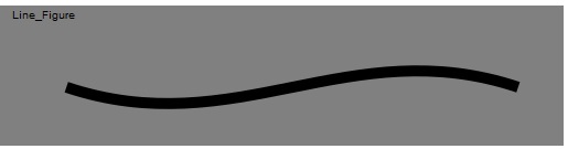
The following is an example to draw a line −
First, we will create a cr context.
julia> using Cairojulia> img = CairoRGBSurface(512, 128);julia> img = CairoRGBSurface(512, 128);julia> cr = CairoContext(img);julia> save(cr);
Now, we will add a rectangle −
julia> set_source_rgb(cr, 0.5, 0.5, 0.5);julia> rectangle(cr, 0.0, 0.0, 512.0, 128.0);julia> fill(cr);julia> restore(cr);julia> save(cr);
Now, we will define the points and draw a line through those points −
julia> x0=61.2; y0=74.0;julia> x1=214.8; y1=125.4;julia> x2=317.2; y2=22.8;julia> x3=470.8; y3=74.0;julia> move_to(cr, x0, y0);julia> curve_to(cr, x1, y1, x2, y2, x3, y3);julia> set_line_width(cr, 10.0);julia> stroke_preserve(cr);julia> restore(cr);
Finally, writing the resulting graphics to the disk −
julia> move_to(cr, 12.0, 12.0);julia> set_source_rgb(cr, 0, 0, 0);julia> show_text(cr,"Line_Figure")julia> write_to_png(c,"Line_Figure.png");
Output
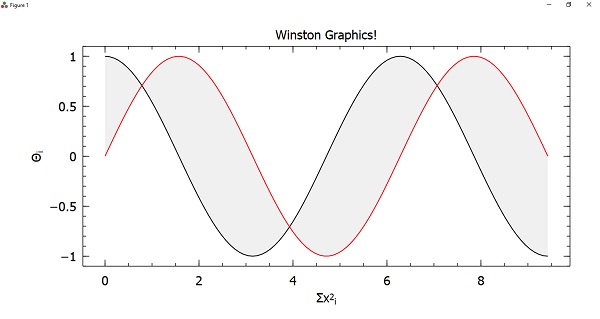
Text Plotting with Winston
Winston is also a 2D graphics library. It resembles the built-in graphics available within MATLAB.
Example
julia> x = range(0, stop=3pi, length=100);julia> c = cos.(x);julia> s = sin.(x);julia> p = FramedPlot( title="Winston Graphics!", xlabel="\\Sigma x^2_i", ylabel="\\Theta_i") julia> add(p, FillBetween(x, c, x, s))julia> add(p, Curve(x, c, color="black"))julia> add(p, Curve(x, s, color="red"))
Output
Data Visualization
Data visualization may be defined as the presentation of data in a variety of graphical as well as pictorial formats such as pie and bar charts.
Gadfly
Gadfly is a powerful Julia package for data visualization and an implementation of the grammar of graphics style. It is based on the same principal as ggplot2 in R. For using it, we need to first add it with the help of Julia package manager.
Example
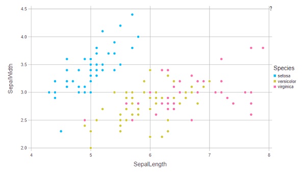
To use Gadfly, we first need to use RDatasets package so that we can get some datasets to work with. In this example, we will be using iris dataset −
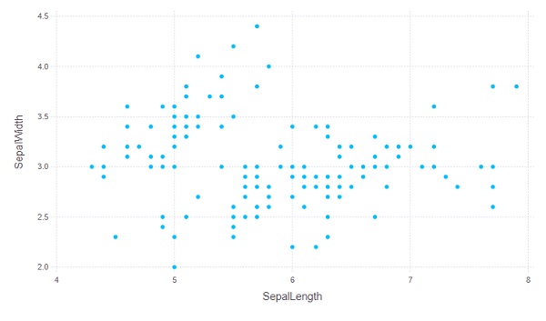
julia> using Gadflyjulia> using RDatasetsjulia> iris = dataset("datasets", "iris");julia> first(iris,10)105 DataFrame Row SepalLength SepalWidth PetalLength PetalWidth Species Float64 Float64 Float64 Float64 Cat 1 5.1 3.5 1.4 0.2 setosa 2 4.9 3.0 1.4 0.2 setosa 3 4.7 3.2 1.3 0.2 setosa 4 4.6 3.1 1.5 0.2 setosa 5 5.0 3.6 1.4 0.2 setosa 6 5.4 3.9 1.7 0.4 setosa 7 4.6 3.4 1.4 0.3 setosa 8 5.0 3.4 1.5 0.2 setosa 9 4.4 2.9 1.4 0.2 setosa 10 4.9 3.1 1.5 0.1 setosa Now let us plot a scatter plot. We will be using the variables namely SepalLength and SepalWidth. For this, we need to set the geometry element using Geom.point as follows −
julia> Gadfly.plot(iris, x = :SepalLength, y = :SepalWidth, Geom.point)
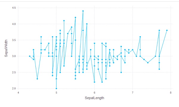
Similarly we can add some more geometries like geom.line to produce more layers in the plot −
julia> Gadfly.plot(iris, x = :SepalLength, y = :SepalWidth, Geom.point, Geom.line)
We can also set the color of keyword argument as follows −
julia> Gadfly.plot(iris, x = :SepalLength, y = :SepalWidth, color = :Species, Geom.point)
Compose
Compose is a declarative vector graphics system. It is also written by Daniel Jones as a part of the Gadfly system. In Compose, the graphics are defined using a tree structure and the primitives can be classified as follows −
Context − It represents an internal node.
Form − It represents a leaf node which defines some geometry such as a circle or line.
Property − It represents a leaf node that modifies how its parents subtree is drawn. For example, fill color and line width.
Compose(x,y) − It returns a new tree rooted at x and with y attached as child.
Example
The below example will draw a simple image −
julia> using Composejulia> composition = compose(compose(context(), rectangle()), fill("tomato"))julia> draw(SVG("simple.svg", 6cm, 6cm), composition)
Now let us form more complex trees by grouping subtrees with brackets −
julia> composition = compose(context(), (context(), circle(), fill("bisque")), (context(), rectangle(), fill("tomato")))julia> composition |> SVG("simple2.svg")
Graphics Engines
In this section, we shall discuss various graphic engines used in Julia.
PyPlot
PyPlot, arose from the previous development of the PyCall module, provides a Julia interface to the Matplotlib plotting library from Python. It uses the PyCall package to call Matplotlib directly from Julia. To work with PytPlot, we need to do the following setup −
julia> using Pkgjulia> pkg"up; add PyPlot Conda"julia> using Condajulia> Conda.add("matplotlib")Once you are done with this setup, you can simply import PyPlot by using PyPlot command. It will let you make calling functions in matplotlib.pyplot.
Example
This example, from PyPlot documentation, will create a sinusoidally modulated sinusoid −
julia> using PyPlotjulia> x = range(0; stop=2*pi, length=500);julia> y = sin.(3 * x + 4 * cos.(2 * x));julia> plot(x, y, color="blue", linewidth=1.0, linestyle="--")1-element Array{PyCall.PyObject,1}:PyObject <matplotlib.lines.Line2D object at 0x00000000323405E0>julia> title("A sinusoidally modulated sinusoid")PyObject Text(0.5, 1.0, 'A sinusoidally modulated sinusoid')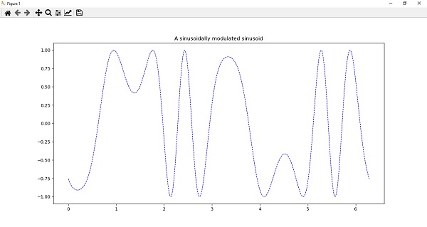
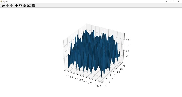
The PyPlot package can also be used for 3d plotting and for this it can import functions from Matplotlibs mplot3d toolkit. We can create 3d plots directly also by calling some corresponding methods such as bar3d, plot_surface, plot3d, etc., of Axes3d.
For example, we can plot a random surface mesh as follows −
julia> surf(rand(20,30))PyObject <mpl_toolkits.mplot3d.art3d.Poly3DCollection object at 0x00000000019BD550>
Gaston
Gaston is another useful package for plotting. This plotting package provides an interface to gnuplot.
Some of the features of Gaston are as follows −
It can plot using graphical windows, and with mouse interaction, it can keep multiple plots active at one time.
It can plot directly to the REPL.
It can also plot in Jupyter and Juno.
It supports popular 2-dimensional plots such as stem, step, histograms, etc.
It also supports popular 3-dimensional plots such as surface, contour, and heatmap.
It takes around five seconds to load package, plot, and save to pdf.
Example
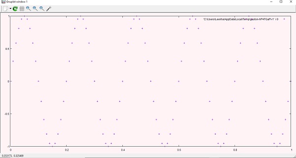
A simple 2-D plot with the help of Gaston is shown below −
julia> x = 0:0.01:10.0:0.01:1.0julia> plot(x, sin.(2*5*t))
Now, we can add another curve as follows −
julia> plot!(x, cos.(2*5*t))
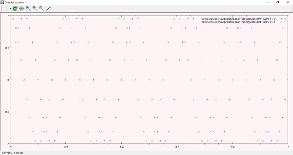
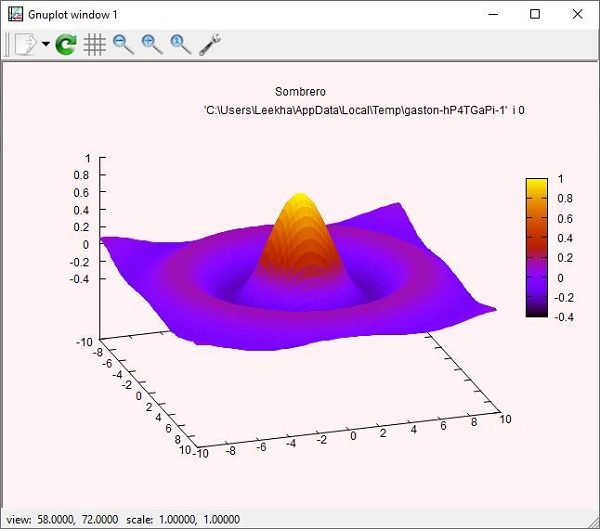
PyPlot can also be used to plot 3-d plots. Example is given below:julia> a = b = -10:0.30:10-10.0:0.3:9.8julia> surf(a, b, (a,b)->sin.(sqrt.(a.*a+b.*b))./sqrt.(a.*a+b.*b), title="Sombrero", plotstyle="pm3d")
PGF Plots
PGFPlots, unlike Gaston, is relatively a new package for plotting. This plotting package uses the pgfplots LaTex routines to produce the plots. It can easily integrate with IJulia, outputting SVG images to notebook. To work with it, we need to install the following dependencies −
Pdf2svg, which is required by TikzPictures.
Pgfplots, which you can install using latex package manager.
GNUPlot, which you need to plot contours
Once you are done with these installations, you are ready to use PGFPlots.
In this example, we will be generating multiple curves on the same axis and assign their legend entries in LaTex format −
julia> using PGFPlotsjulia> R = Axis( [ Plots.Linear(x->sin(3x)*exp(-0.3x), (0,8), legendentry = L"$\sin(3x)*exp(-0.3x)$"), Plots.Linear(x->sqrt(x)/(1+x^2), (0,8), legendentry = L"$\sqrt{2x}/(1+x^2)$") ]); julia> save("Plot_LinearPGF.svg", R); 