Julia Programming - Data Frames

Quiz

DataFrame may be defined as a table or spreadsheet which we can be used to sort as well as explore a set of related data values. In other words, we can call it a smarter array for holding tabular data. Before we use it, we need to download and install DataFrame and CSV packages as follows −

(@v1.5) pkg> add DataFrames(@v1.5) pkg> add CSV

To start using the DataFrames package, type the following command −

julia> using DataFrames

Loading data into DataFrames

There are several ways to create new DataFrames (which we will discuss later in this section) but one of the quickest ways to load data into DataFrames is to load the Anscombe dataset. For better understanding, let us see the example below −

anscombe = DataFrame(         [10 10 10 8 8.04 9.14 7.46 6.58;           8 8   8 8 6.95 8.14 6.77 5.76;          13 13 13 8 7.58 8.74 12.74 7.71;           9 9   9 8 8.81 8.77 7.11 8.84;          11 11 11 8 8.33 9.26 7.81 8.47;          14 14 14 8 9.96 8.1  8.84 7.04;           6 6   6 8 7.24 6.13 6.08 5.25;           4 4   4 19 4.26 3.1 5.39 12.5;          12 12 12 8 10.84 9.13 8.15 5.56;           7 7   7 8 4.82  7.26 6.42 7.91;           5 5   5 8 5.68 4.74 5.73 6.89]);

julia> rename!(anscombe, [Symbol.(:N, 1:4); Symbol.(:M, 1:4)])118 DataFrame Row     N1       N2      N3        N4       M1        M2       M3      M4         Float64  Float64  Float64  Float64  Float64  Float64  Float64  Float64  1    10.0     10.0     10.0     8.0      8.04     9.14     7.46     6.58     2    8.0      8.0      8.0      8.0      6.95     8.14     6.77     5.76     3    13.0     13.0     13.0     8.0      7.58     8.74     12.74    7.71     4    9.0      9.0      9.0      8.0      8.81     8.77     7.11     8.84     5    11.0     11.0     11.0     8.0      8.33     9.26     7.81     8.47     6    14.0     14.0     14.0     8.0      9.96     8.1      8.84     7.04     7    6.0      6.0      6.0      8.0      7.24     6.13     6.08     5.25     8    4.0      4.0      4.0      19.0     4.26     3.1      5.39     12.5     9    12.0     12.0     12.0     8.0      10.84    9.13     8.15     5.56    10    7.0      7.0      7.0      8.0      4.82     7.26     6.42     7.91    11    5.0      5.0      5.0      8.0      5.68     4.74     5.73     6.89

We assigned the DataFrame to a variable named Anscombe, convert them to an array and then rename columns.

Collected Datasets

We can also use another dataset package named RDatasets package. It contains several other famous datasets including Anscombes. Before we start using it, we need to first download and install it as follows −

(@v1.5) pkg> add RDatasets

To start using this package, type the following command −

julia> using DataFramesjulia> anscombe = dataset("datasets","anscombe")118 DataFrame Row    X1     X2     X3     X4     Y1        Y2       Y3      Y4          Int64  Int64  Int64  Int64  Float64  Float64  Float64  Float64  1     10      10      10   8       8.04    9.14       7.46  6.58     2     8       8       8    8       6.95    8.14       6.77  5.76     3     13      13      13   8       7.58    8.74       12.74 7.71     4     9       9       9    8       8.81    8.77       7.11  8.84     5     11      11      11   8       8.33    9.26       7.81  8.47     6     14      14      14   8       9.96    8.1        8.84  7.04     7     6       6       6    8       7.24    6.13       6.08  5.25     8     4       4       4    19      4.26    3.1        5.39  12.5     9     12      12      12   8       10.84   9.13       8.15  5.56     10    7       7       7    8       4.82    7.26       6.42  7.91     11    5       5       5    8       5.68    4.74       5.73  6.89

Empty DataFrames

We can also create DataFrames by simply providing the information about rows, columns as we give in an array.

Example

julia> empty_df = DataFrame(X = 1:10, Y = 21:30)102 DataFrame Row    X      Y         Int64  Int64  1       1     21   2       2     22   3       3     23   4       4     24   5       5     25   6       6     26   7       7     27   8       8     28   9       9     29   10     10     30

To create completely empty DataFrame, we only need to supply the Column Names and define their types as follows −

julia> Complete_empty_df = DataFrame(Name=String[],         W=Float64[],         H=Float64[],         M=Float64[],         V=Float64[])05 DataFrame

julia> Complete_empty_df = vcat(Complete_empty_df, DataFrame(Name="EmptyTestDataFrame", W=5.0, H=5.0, M=3.0, V=5.0))15 DataFrame Row      Name                W       H       M          V             String          Float64  Float64  Float64  Float64  1    EmptyTestDataFrame   5.0        5.0     3.0        5.0

julia> Complete_empty_df = vcat(Complete_empty_df, DataFrame(Name="EmptyTestDataFrame2", W=6.0, H=6.0, M=5.0, V=7.0))25 DataFrame Row         Name             W       H          M       V                 String        Float64  Float64  Float64  Float64  1    EmptyTestDataFrame      5.0     5.0     3.0        5.0   2    EmptyTestDataFrame2     6.0     6.0     5.0        7.0

Plotting Anscombes Quarter

Now the Anscombe dataset has been loaded, we can do some statistics with it also. The inbuilt function named describe() enables us to calculate the statistics properties of the columns of a dataset. You can supply the symbols, given below, for the properties −

mean
std
min
q25
median
q75
max
eltype
nunique
first
last
nmissing

Example

julia> describe(anscombe, :mean, :std, :min, :median, :q25)86 DataFrame Row  variable    mean       std  min    median    q25          Symbol   Float64  Float64  Real  Float64  Float64   1       X1      9.0    3.31662     4    9.0     6.5      2       X2      9.0    3.31662     4    9.0     6.5      3       X3      9.0    3.31662     4    9.0     6.5      4       X4      9.0    3.31662     8    8.0     8.0      5       Y1    7.50091  2.03157  4.26    7.58   6.315     6       Y2    7.50091  2.03166  3.1     8.14   6.695     7       Y3      7.5    2.03042  5.39    7.11   6.25      8       Y4    7.50091  2.03058  5.25    7.04   6.17

We can also do a comparison between XY datasets as follows −

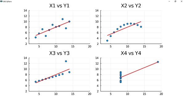
julia> [describe(anscombe[:, xy], :mean, :std, :median, :q25) for xy in [[:X1, :Y1], [:X2, :Y2], [:X3, :Y3], [:X4, :Y4]]]4-element Array{DataFrame,1}:25 DataFrame Row  variable    mean       std   median    q25          Symbol   Float64  Float64  Float64  Float64  1      X1        9.0    3.31662     9.0     6.5    2     Y1       7.50091  2.03157     7.58  6.315   25 DataFrame Row  variable    mean    std     median     q25          Symbol   Float64  Float64  Float64  Float64  1        X2       9.0   3.31662     9.0       6.5  2        Y2    7.50091  2.03166     8.14    6.695 25 DataFrame Row  variable    mean       std   median    q25          Symbol   Float64  Float64  Float64  Float64  1        X3        9.0  3.31662     9.0     6.5    2        Y3        7.5  2.03042     7.11    6.25  25 DataFrame Row  variable    mean    std      median    q25          Symbol   Float64  Float64  Float64  Float64  1        X4      9.0    3.31662     8.0     8.0    2        Y4    7.50091  2.03058     7.04    6.17

Let us reveal the true purpose of Anscombe, i.e., plot the four sets of its quartet as follows −

julia> using StatsPlots[ Info: Precompiling StatsPlots [f3b207a7-027a-5e70-b257-86293d7955fd]julia> @df anscombe scatter([:X1 :X2 :X3 :X4], [:Y1 :Y2 :Y3 :Y4],            smooth=true,            line = :red,            linewidth = 2,            title= ["X$i vs Y$i" for i in (1:4)'],            legend = false,            layout = 4,            xlimits = (2, 20),            ylimits = (2, 14))

Regression and Models

In this section, we will be working with Linear Regression line for the dataset. For this we need to use Generalized Linear Model (GLM) package which you need to first add as follows −

(@v1.5) pkg> add GLM

Now let us create a liner regression model by specifying a formula using the @formula macro and supplying columns names as well as name of the DataFrame. An example for the same is given below −

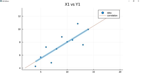
julia> linearregressionmodel = fit(LinearModel, @formula(Y1 ~ X1), anscombe)StatsModels.TableRegressionModel{LinearModel{GLM.LmResp{Array{Float64,1}},GLM.DensePredChol{Float64,LinearAlgebra.Cholesky{Float64,Array{Float64,2}}}},Array{Float64,2}}Y1 ~ 1 + X1Coefficients:               Coef.    Std.     Error    t Pr(>|t|) Lower 95% Upper 95%(Intercept) 3.00009  1.12475     2.67     0.0257      0.455737  5.54444   X1       0.500091 0.117906    4.24     0.0022      0.23337   0.766812

Let us check the summary and the coefficient of the above created linear regression model −

julia> summary(linearregressionmodel)"StatsModels.TableRegressionModel{LinearModel{GLM.LmResp{Array{Float64,1}},GLM.DensePredChol{Float64,LinearAlgebra.Cholesky{Float64,Array{Float64,2}}}},Array{Float64,2}}"julia> coef(linearregressionmodel)2-element Array{Float64,1}: 3.0000909090909054 0.5000909090909096

Now let us produce a function for the regression line. The form of the function is y = ax +c.

julia> f(x) = coef(linearmodel)[2] * x + coef(linearmodel)[1]f (generic function with 1 method)

Once we have the function that describes the regression line, we can draw a plot as follows −

julia> p1 = plot(anscombe[:X1], anscombe[:Y1],            smooth=true,            seriestype=:scatter,            title = "X1 vs Y1",            linewidth=8,            linealpha=0.5,            label="data")            julia> plot!(f, 2, 20, label="correlation")

Working with DataFrames

As we know that nothing is perfect. This is also true in case of datasets because not all the datasets are consistent and tidy. To show how we can work with different items of DataFrame, let us create a test DataFrame −

julia> testdf = DataFrame( Number = [3, 5, 7, 8, 20 ],                             Name = ["Lithium", "Boron", "Nitrogen", "Oxygen", "Calcium" ],                     AtomicWeight = [6.941, 10.811, 14.0067, 15.9994, 40.078 ],                           Symbol = ["Li", "B", "N", "O", "Ca" ],                       Discovered = [1817, 1808, 1772, 1774, missing ])55 DataFrame Row  Number      Name  AtomicWeight  Symbol  Discovered        Int64   String        Float64  String    Int64?     1       3   Lithium        6.941        Li    1817       2       5    Boron         10.811       B     1808       3       7   Nitrogen       14.0067      N     1772       4       8    Oxygen        15.9994      O     1774       5       20  Calcium        40.078       Ca    missing

Handling missing values

There can be some missing values in datasets. It can be checked with the help of describe() function as follows −

julia> describe(testdf)58 DataFrame Row      variable   mean    min    median      max  nunique  nmissing         eltype                   Symbol     Union  Any    Union      Any  Union   Union           Type             1       Number     8.6        3    7.0        20                            Int64             2       Name               Boron           Oxygen     5                     String            3   AtomicWeight  17.5672  6.941  14.0067  40.078                           Float64           4   Symbol                    B                 O     5                     String            5   Discovered    1792.75  1772   1791.0     1817               1     Union{Missing, Int64}

Julia provides a special datatype called Missing to address such issue. This datatype indicates that there is not a usable value at this location. That is why the DataFrames packages allow us to get most of our datasets and make sure that the calculations are not tampered due to missing values.

Looking for missing values

We can check with ismissing() function that whether the DataFrame has any missing value or not.

Example

julia> for row in 1:nrows            for col in 1:ncols               if ismissing(testdf [row,col])                  println("$(names(testdf)[col]) value for $(testdf[row,:Name]) is missing!")               end            end         end

Discovered value for Calcium is missing!

Repairing DataFrames

We can use the following code to change values that are not acceptable like n/a, 0, missing. The below code will look in every cell for above mentioned non-acceptable values.

Example

julia> for row in 1:size(testdf, 1) # or nrow(testdf)         for col in 1:size(testdf, 2) # or ncol(testdf)            println("processing row $row column $col ")            temp = testdf [row,col]            if ismissing(temp)               println("skipping missing")            elseif temp == "n/a" || temp == "0" || temp == 0               testdf [row, col] = missing               println("changed row $row column $col ")            end         end      endprocessing row 1 column 1processing row 1 column 2processing row 1 column 3processing row 1 column 4processing row 1 column 5processing row 2 column 1processing row 2 column 2processing row 2 column 3processing row 2 column 4processing row 2 column 5processing row 3 column 1processing row 3 column 2processing row 3 column 3processing row 3 column 4processing row 3 column 5processing row 4 column 1processing row 4 column 2processing row 4 column 3processing row 4 column 4processing row 4 column 5processing row 5 column 1processing row 5 column 2processing row 5 column 3processing row 5 column 4processing row 5 column 5skipping missing

Working with missing values

Julia provides support for representing missing values in the statistical sense, that is for situations where no value is available for a variable in an observation, but a valid value theoretically exists.

completecases()

The completecases() function is used to find the maximum value of the column that contains the missing value.

Example

julia> maximum(testdf[completecases(testdf), :].Discovered)1817

dropmissing()

The dropmissing() function is used to get the copy of DataFrames without having the missing values.

Example

julia> dropmissing(testdf)45 DataFrame Row  Number     Name   AtomicWeight  Symbol  Discovered       Int64    String     Float64     String     Int64     1    3      Lithium       6.941       Li      1817       2    5       Boron      10.811         B      1808       3    7      Nitrogen    14.0067        N      1772       4    8       Oxygen     15.9994        O      1774

Modifying DataFrames

The DataFrames package of Julia provides various methods using which you can add, remove, rename columns, and add/delete rows.

Adding Columns

We can use hcat() function to add a column of integers to the DataFrame. It can be used as follows −

julia> hcat(testdf, axes(testdf, 1))56 DataFrame Row  Number      Name  AtomicWeight  Symbol  Discovered   x1         Int64     String    Float64     String    Int64?    Int64   1    3       Lithium       6.941      Li      1817        1     2    5         Boron       10.811     B        1808       2     3    7      Nitrogen       14.0067    N        1772       3     4    8        Oxygen       15.9994    O       1774        4     5    20      Calcium       40.078     Ca      missing     5

But as you can notice that we havent changed the DataFrame or assigned any new DataFrame to a symbol. We can add another column as follows −

julia> testdf [!, :MP] = [180.7, 2300, -209.86, -222.65, 839]5-element Array{Float64,1}: 180.7 2300.0 -209.86 -222.65 839.0julia> testdf56 DataFrame Row  Number     Name   AtomicWeight  Symbol  Discovered    MP           Int64   String     Float64     String    Int64?    Float64   1       3    Lithium       6.941      Li       1817     180.7     2       5    Boron         10.811      B       1808     2300.0    3       7   Nitrogen       14.0067    N        1772     -209.86   4       8     Oxygen       15.9994    O        1774     -222.65   5       20   Calcium       40.078     Ca       missing  839.0

We have added a column having melting points of all the elements to our test DataFrame.

Removing Columns

We can use select!() function to remove a column from the DataFrame. It will create a new DataFrame that contains the selected columns, hence to remove a particular column, we need to use select!() with Not. It is shown in the given example −

julia> select!(testdf, Not(:MP))55 DataFrame Row  Number   Name     AtomicWeight  Symbol  Discovered       Int64   String      Float64     String    Int64?     1       3   Lithium        6.941      Li      1817       2       5    Boron         10.811     B       1808       3       7   Nitrogen       14.0067    N       1772       4       8    Oxygen        15.9994    O       1774       5       20  Calcium        40.078     Ca      missing

We have removed the column MP from our Data Frame.

Renaming Columns

We can use rename!() function to rename a column in the DataFrame. We will be renaming the AtomicWeight column to AW as follows −

julia> rename!(testdf, :AtomicWeight => :AW)55 DataFrame Row  Number  Name        AW     Symbol  Discovered       Int64   String    Float64  String   Int64?      1     3      Lithium  6.941     Li         1817     2     5        Boron  10.811    B          1808     3     7     Nitrogen  14.0067   N          1772     4     8      Oxygen   15.9994   O          1774     5    20      Calcium  40.078    Ca      missing

Adding rows

We can use push!() function with suitable data to add rows in the DataFrame. In the below given example we will be adding a row having element Cooper −

Example

julia> push!(testdf, [29, "Copper", 63.546, "Cu", missing])65 DataFrame Row  Number     Name        AW  Symbol  Discovered        Int64   String   Float64  String     Int64?    1       3    Lithium    6.941      Li      1817     2       5      Boron   10.811       B      1808     3       7   Nitrogen  14.0067       N       1772    4       8    Oxygen   15.9994       O       1774    5       20   Calcium   40.078      Ca    missing    6       29   Copper    63.546      Cu   missing

Deleting rows

We can use deleterows!() function with suitable data to delete rows from the DataFrame. In the below given example we will be deleting three rows (4th, 5th,and 6th) from our test data frame −

Example

julia> deleterows!(testdf, 4:6)35 DataFrame Row  Number   Name       AW     Symbol  Discovered        Int64  String    Float64  String   Int64?      1    3       Lithium    6.941   Li      1817        2    5         Boron   10.811   B       1808        3    7      Nitrogen  14.0067   N       1772

Finding values in DataFrame

To find the values in DataFrame, we need to use an elementwise operator examining all the rows. This operator will return an array of Boolean values to indicate whether cells meet the criteria or not.

Example

julia> testdf[:, :AW] .< 103-element BitArray{1}:100julia> testdf[testdf[:, :AW] .< 10, :]15 DataFrame Row  Number    Name        AW  Symbol  Discovered        Int64   String  Float64  String    Int64?    1       3    Lithium  6.941      Li      1817

Sorting

To sort the values in DataFrame, we can use sort!() function. We need to give the columns on which we want to sort.

Example

julia> sort!(testdf, [order(:AW)])35 DataFrame Row  Number   Name       AW     Symbol  Discovered        Int64  String    Float64  String   Int64?     1     3      Lithium     6.941   Li         1817    2     5       Boron     10.811   B          1808    3     7      Nitrogen  14.0067   N          1772

The DataFrame is sorted based on the values of column AW.

Print Page