How to use TOCOL and TOROW functions in Excel?

Microsoft Excel 365 comprises a wide range of new functions to improve users' productivity and efficiency in manipulating data. With big datasets, it takes a lot of time for users to manually transform a 2-D array into a single array. TOCOL and TOROW functions are new inbuilt functions introduced in Excel 365 that are used to rebuild a two-dimensional array into a one-dimensional array. These functions are opposite to WRAPROWS and WRAPCOLS functions. TOCOL streamlines the data values vertically whereas TOROW visualizes the cell’s values only in a single row.

Implementation of TOCOL Function in Excel

Step 1

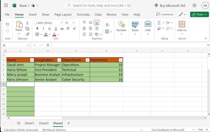
Open a new worksheet in Excel 365 and enter the sample data as shown below −

Step 2

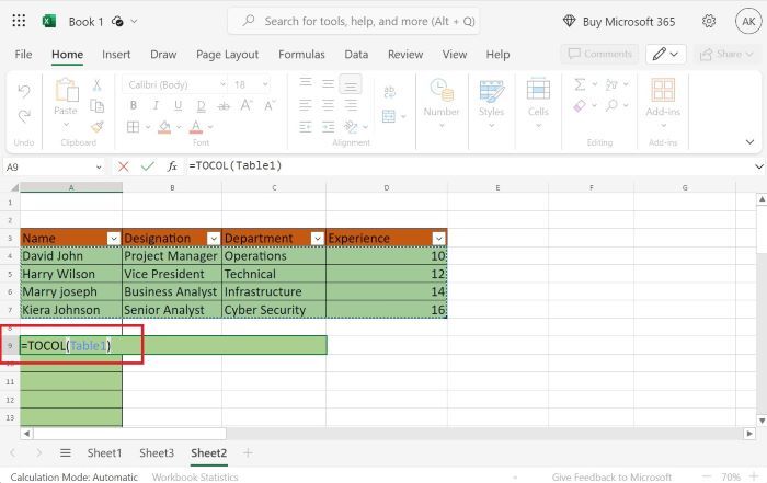
Write the formula “=TOCOL(Table1)” in the “A9” cell as illustrated below −

Syntax of TOCOL Function

=TOCOL(arr, [ignore], [scan_col])

Three arguments are defined in the TOCOL function definition −

• arr − Users must specify a certain range for the table.

• ignore − It is an optional argument. Its values range from 0 to 3. By default, 0 will be used. 1 means blanks that exist in the dataset will be avoided. 2 means errors will be avoided in the array. The number 3 indicates the blanks, as well as faults, will be avoided.

• scan_col − It is also an optional argument. It identifies whether the scanning of data is column-wise or row-wise.

Step 3

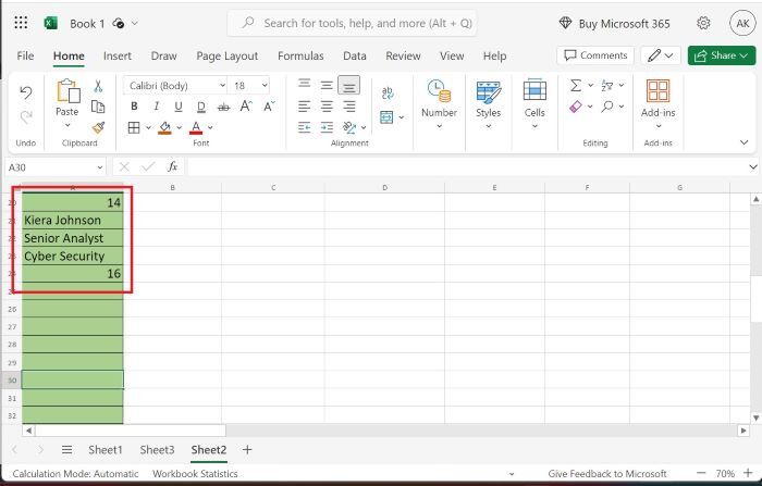
Press the “Enter” tab and the result is displayed in one column as highlighted below image −

Execution of TOROWS Function in Excel

Step 1

Consider the sample dataset as given below −

Step 2

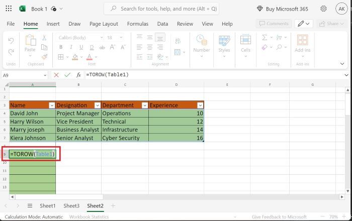
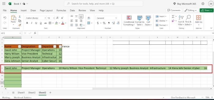
Write the formula “=TOROW(TABLE1)” in the A9 cell.

Syntax of TOROW Function

=TOROW(arr, [ignore], [scan_row])

The three arguments to be defined in the function definition −

• arr − Users intend to specify the range of the table.

• ignore − It is an optional argument. By default, 0 values will be considered to retain all entries. To skip empty cell values, 1 number is to be specified. To avoid errors presented in the array, users need to specify 2 numbers in this argument. To avoid faults and empty values, the number 3 is to be defined.

• scan_row − By default, the data values will be scanned row-wise. It is also an optional argument.

Step 3

Then press the “Enter” tab to display the result as illustrated below −

Conclusion

In this article, by utilizing the TOCOL and TOROW functions, we can quickly pile the data values either horizontally (single row) or vertically (single column). Users can acquire a thorough knowledge of their data by organizing their data across many ranges in worksheets.