How to Calculate the Impulse Response in MATLAB?

In this article, we will learn ow to calculate the impulse response of a system in MATLAB. Impulse response is an elementary concept used in analyzing and understanding the behavior of systems for an impulse input.

It is mainly used to analyze the linear time invariant systems like digital filters, electronic circuits, signal processing systems, control systems, and more.

Impulse response of a system can be defined as follows:

The response of a system when an impulse input signal is applied to it, is called the impulse response. It is denoted as h(t) for continuous time systems and h[n] for discrete time systems.

Impulse response used to specify the response of a system to an impulse input signal in the time domain. Where, an impulse signal is a signal of infinite magnitude and infinitesimally small in time.

Mathematically, the impulse signal is expressed as follows:

For continuous time systems (CTS)

$$\mathrm{\delta(t)\:=\:0;\:for\:t
eq 0}$$

$$\mathrm{\int_{−\infty}^{\infty}\delta(t)dt\:=\:1}$$

For discrete time systems (DTS)

$$\mathrm{\delta[n]\:=\:0;\:for\:n
eq 0}$$

$$\mathrm{\sum_{−\infty}^{\infty} \delta[n]\:=\:1}$$

Overall, the impulse response of a system allows us to analyze and study the system behavior for its stability, time domain properties, frequency response, etc.

Algorithm to Calculate Impulse Response in MATLAB

The step−by−step procedure to calculate the impulse response of a system in MATLAB is described below:

Step (1) − Define a system either by through the transfer function of the system or by its difference equation.

Step (2) − Compute the impulse response of the system by using the MATLAB’s built−in function named, ‘impulse’.

Step (3) − Plot the impulse response of the system by using the ‘plot’ function. This step visualizes the impulse response graphically.

Now, let us consider a few example programs in MATLAB to calculate and visualize the impulse response of systems.

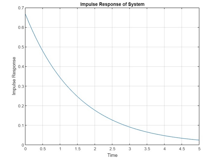
Example (1) − Impulse Response of a First−Order System

The following MATLAB program demonstrates the calculation and visualization of the impulse response of a first order system.

Let the following is the transfer function representing a first−order system:

$$\mathrm{H(s)\:=\:\frac{2}{3s+2}}$$

Example

% MATLAB code for computing the impulse Response of a second-order digital filter
% Specify the difference equation coefficients of the filter
ff = [0.7, 0.35, 0.55];	% Feedforward coefficients
fb = 1;			% Feedback coefficient i.e., no feedback
% Create a sample vector
n = 0:5;	% Adjust as per need
% Compute the impulse response of the system
h = impz(ff, fb, n);
% Plot the impulse response
stem(n, h); title('Impulse Response of Second-Order Digital Filter');
xlabel('Sample Index (n)');
ylabel('Impulse Response');
grid on;

Output

Code Explanation

In this MATLAB program, we start by defining the transfer function of a first order system. Then, we create a transfer function model of the system. Next, we calculate the impulse response of the system by using the ‘impulse’ function. Finally, we plot the impulse response of the system using the ‘plot’ function.

Example (2) − Impulse Response of the Second−Order Recursive Digital Filter

The following MATLAB program demonstrates the calculation of the impulse response of a second−order recursive digital filter with infinite impulse response.

Let the following difference equation represents the digital filter:

r[n] = 0.7c[n]+0.35c[n−1]+0.55c[n−2]

Example

% MATLAB code for computing the impulse Response of a second-order digital filter
% Specify the difference equation coefficients of the filter
ff = [0.7, 0.35, 0.55];	% Feedforward coefficients
fb = 1;			% Feedback coefficient i.e., no feedback
% Create a sample vector
n = 0:5;	% Adjust as per need
% Compute the impulse response of the system
h = impz(ff, fb, n);
% Plot the impulse response
stem(n, h); title('Impulse Response of Second-Order Digital Filter');
xlabel('Sample Index (n)');
ylabel('Impulse Response');
grid on;

Output

Code Explanation

In this MATLAB program, we start by defining the transfer function of a first order system. Then, we create a transfer function model of the system. Next, we calculate the impulse response of the system by using the ‘impulse’ function. Finally, we plot the impulse response of the system using the ‘plot’ function.

Conclusion

Hence, this is all about calculating the impulse response of a system using MATLAB. MATLAB provides two built−in functions namely, ‘impulse’ and ‘impz’ to compute the impulse response of a continuous−time system and discrete−time system respectively. The above example programs illustrate the utilization of these function to compute the impulse response.