- H2O - Home
- H2O - Introduction
- H2O - Installation
- H2O - Flow
- H2O - Running Sample Application
- H2O - AutoML
- H2O Useful Resources
- H2O - Quick Guide
- H2O - Useful Resources
- H2O - Discussion
H2O - Running Sample Application
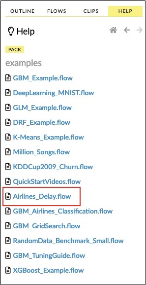
Click on the Airlines Delay Flow link in the list of samples as shown in the screenshot below −
After you confirm, the new notebook would be loaded.
Clearing All Outputs
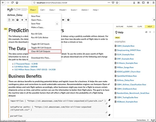
Before we explain the code statements in the notebook, let us clear all the outputs and then run the notebook gradually. To clear all outputs, select the following menu option −
Flow / Clear All Cell Contents
This is shown in the following screenshot −
Once all outputs are cleared, we will run each cell in the notebook individually and examine its output.
Running the First Cell
Click the first cell. A red flag appears on the left indicating that the cell is selected. This is as shown in the screenshot below −
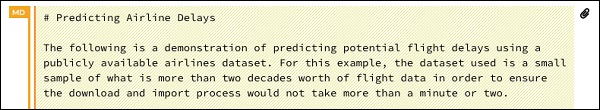
The contents of this cell are just the program comment written in MarkDown (MD) language. The content describes what the loaded application does. To run the cell, click the Run icon as shown in the screenshot below −

You will not see any output underneath the cell as there is no executable code in the current cell. The cursor now moves automatically to the next cell, which is ready to execute.
Importing Data
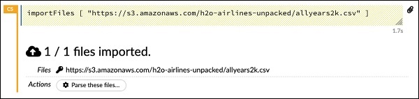
The next cell contains the following Python statement −
importFiles ["https://s3.amazonaws.com/h2o-airlines-unpacked/allyears2k.csv"]
The statement imports the allyears2k.csv file from Amazon AWS into the system. When you run the cell, it imports the file and gives you the following output.
Setting Up Data Parser
Now, we need to parse the data and make it suitable for our ML algorithm. This is done using the following command −
setupParse paths: [ "https://s3.amazonaws.com/h2o-airlines-unpacked/allyears2k.csv" ]
Upon execution of the above statement, a setup configuration dialog appears. The dialog allows you several settings for parsing the file. This is as shown in the screenshot below −
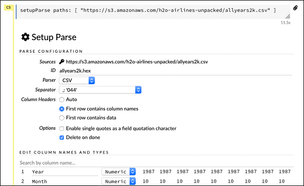
In this dialog, you can select the desired parser from the given drop-down list and set other parameters such as the field separator, etc.
Parsing Data
The next statement, which actually parses the datafile using the above configuration, is a long one and is as shown here −
parseFiles
paths: ["https://s3.amazonaws.com/h2o-airlines-unpacked/allyears2k.csv"]
destination_frame: "allyears2k.hex"
parse_type: "CSV"
separator: 44
number_columns: 31
single_quotes: false
column_names: ["Year","Month","DayofMonth","DayOfWeek","DepTime","CRSDepTime",
   "ArrTime","CRSArrTime","UniqueCarrier","FlightNum","TailNum",
   "ActualElapsedTime","CRSElapsedTime","AirTime","ArrDelay","DepDelay",
   "Origin","Dest","Distance","TaxiIn","TaxiOut","Cancelled","CancellationCode",
   "Diverted","CarrierDelay","WeatherDelay","NASDelay","SecurityDelay",
   "LateAircraftDelay","IsArrDelayed","IsDepDelayed"]
column_types: ["Enum","Enum","Enum","Enum","Numeric","Numeric","Numeric"
   ,"Numeric","Enum","Enum","Enum","Numeric","Numeric","Numeric","Numeric",
   "Numeric","Enum","Enum","Numeric","Numeric","Numeric","Enum","Enum",
   "Numeric","Numeric","Numeric","Numeric","Numeric","Numeric","Enum","Enum"]
delete_on_done: true
check_header: 1
chunk_size: 4194304
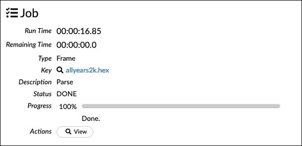
Observe that the parameters you have set up in the configuration box are listed in the above code. Now, run this cell. After a while, the parsing completes and you will see the following output −
Examining Dataframe
After the processing, it generates a dataframe, which can be examined using the following statement −
getFrameSummary "allyears2k.hex"
Upon execution of the above statement, you will see the following output −
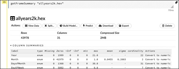
Now, your data is ready to be fed into a Machine Learning algorithm.
The next statement is a program comment that says we will be using the regression model and specifies the preset regularization and the lambda values.
Building the Model
Next, comes the most important statement and that is building the model itself. This is specified in the following statement −
buildModel 'glm', {
   "model_id":"glm_model","training_frame":"allyears2k.hex",
   "ignored_columns":[
      "DayofMonth","DepTime","CRSDepTime","ArrTime","CRSArrTime","TailNum",
      "ActualElapsedTime","CRSElapsedTime","AirTime","ArrDelay","DepDelay",
      "TaxiIn","TaxiOut","Cancelled","CancellationCode","Diverted","CarrierDelay",
      "WeatherDelay","NASDelay","SecurityDelay","LateAircraftDelay","IsArrDelayed"],
   "ignore_const_cols":true,"response_column":"IsDepDelayed","family":"binomial",
   "solver":"IRLSM","alpha":[0.5],"lambda":[0.00001],"lambda_search":false,
   "standardize":true,"non_negative":false,"score_each_iteration":false,
   "max_iterations":-1,"link":"family_default","intercept":true,
   "objective_epsilon":0.00001,"beta_epsilon":0.0001,"gradient_epsilon":0.0001,
   "prior":-1,"max_active_predictors":-1
}
We use glm, which is a Generalized Linear Model suite with family type set to binomial. You can see these highlighted in the above statement. In our case, the expected output is binary and that is why we use the binomial type. You may examine the other parameters by yourself; for example, look at alpha and lambda that we had specified earlier. Refer to the GLM model documentation for the explanation of all the parameters.
Now, run this statement. Upon execution, the following output will be generated −
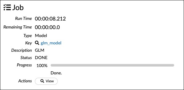
Certainly, the execution time would be different on your machine. Now, comes the most interesting part of this sample code.
Examining Output
We simply output the model that we have built using the following statement −
getModel "glm_model"
Note the glm_model is the model ID that we specified as model_id parameter while building the model in the previous statement. This gives us a huge output detailing the results with several varying parameters. A partial output of the report is shown in the screenshot below −
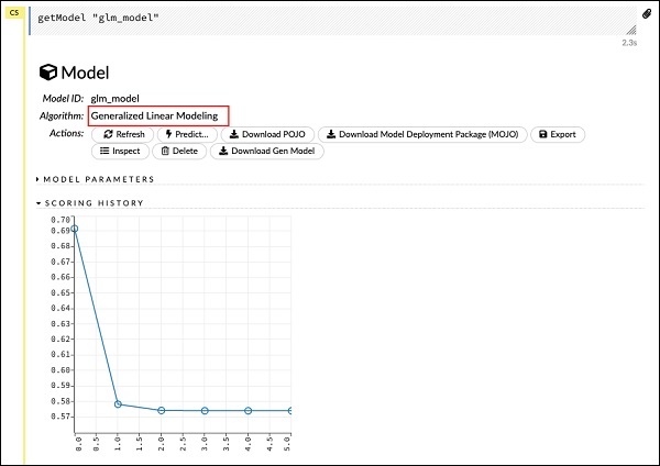
As you can see in the output, it says that this is the result of running the Generalized Linear Modeling algorithm on your dataset.
Right above the SCORING HISTORY, you see the MODEL PARAMETERS tag, expand it and you will see the list of all parameters that are used while building the model. This is shown in the screenshot below.
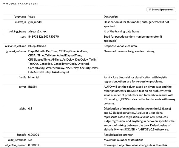
Likewise, each tag provides a detailed output of a specific type. Expand the various tags yourself to study the outputs of different kinds.
Building Another Model
Next, we will build a Deep Learning model on our dataframe. The next statement in the sample code is just a program comment. The following statement is actually a model building command. It is as shown here −
buildModel 'deeplearning', {
   "model_id":"deeplearning_model","training_frame":"allyear
   s2k.hex","ignored_columns":[
      "DepTime","CRSDepTime","ArrTime","CRSArrTime","FlightNum","TailNum",
      "ActualElapsedTime","CRSElapsedTime","AirTime","ArrDelay","DepDelay",
      "TaxiIn","TaxiOut","Cancelled","CancellationCode","Diverted",
      "CarrierDelay","WeatherDelay","NASDelay","SecurityDelay",
      "LateAircraftDelay","IsArrDelayed"],
   "ignore_const_cols":true,"res   ponse_column":"IsDepDelayed",
   "activation":"Rectifier","hidden":[200,200],"epochs":"100",
   "variable_importances":false,"balance_classes":false,
   "checkpoint":"","use_all_factor_levels":true,
   "train_samples_per_iteration":-2,"adaptive_rate":true,
   "input_dropout_ratio":0,"l1":0,"l2":0,"loss":"Automatic","score_interval":5,
   "score_training_samples":10000,"score_duty_cycle":0.1,"autoencoder":false,
   "overwrite_with_best_model":true,"target_ratio_comm_to_comp":0.02,
   "seed":6765686131094811000,"rho":0.99,"epsilon":1e-8,"max_w2":"Infinity",
   "initial_weight_distribution":"UniformAdaptive","classification_stop":0,
   "diagnostics":true,"fast_mode":true,"force_load_balance":true,
   "single_node_mode":false,"shuffle_training_data":false,"missing_values_handling":
   "MeanImputation","quiet_mode":false,"sparse":false,"col_major":false,
   "average_activation":0,"sparsity_beta":0,"max_categorical_features":2147483647,
   "reproducible":false,"export_weights_and_biases":false
}
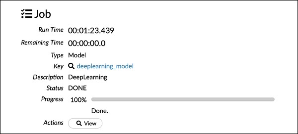
As you can see in the above code, we specify deeplearning for building the model with several parameters set to the appropriate values as specified in the documentation of deeplearning model. When you run this statement, it will take longer time than the GLM model building. You will see the following output when the model building completes, albeit with different timings.
Examining Deep Learning Model Output
This generates the kind of output, which can be examined using the following statement as in the earlier case.
getModel "deeplearning_model"
We will consider the ROC curve output as shown below for quick reference.
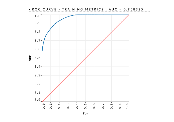
Like in the earlier case, expand the various tabs and study the different outputs.
Saving the Model
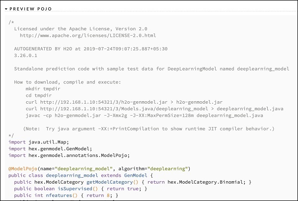
After you have studied the output of different models, you decide to use one of those in your production environment. H20 allows you to save this model as a POJO (Plain Old Java Object).
Expand the last tag PREVIEW POJO in the output and you will see the Java code for your fine-tuned model. Use this in your production environment.
Next, we will learn about a very exciting feature of H2O. We will learn how to use AutoML to test and rank various algorithms based on their performance.
