H2O - Installation

H2O can be configured and used with five different options as listed below −

Install in Python
Install in R
Web-based Flow GUI
Hadoop
Anaconda Cloud

In our subsequent sections, you will see the instructions for installation of H2O based on the options available. You are likely to use one of the options.

Install in Python

To run H2O with Python, the installation requires several dependencies. So let us start installing the minimum set of dependencies to run H2O.

Installing Dependencies

To install a dependency, execute the following pip command −

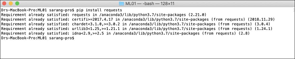
$ pip install requests

Open your console window and type the above command to install the requests package. The following screenshot shows the execution of the above command on our Mac machine −

After installing requests, you need to install three more packages as shown below −

$ pip install tabulate
$ pip install "colorama >= 0.3.8"
$ pip install future

The most updated list of dependencies is available on H2O GitHub page. At the time of this writing, the following dependencies are listed on the page.

python 2. H2O — Installation
pip >= 9.0.1
setuptools
colorama >= 0.3.7
future >= 0.15.2

Removing Older Versions

After installing the above dependencies, you need to remove any existing H2O installation. To do so, run the following command −

$ pip uninstall h2o

Installing the Latest Version

Now, let us install the latest version of H2O using the following command −

$ pip install -f http://h2o-release.s3.amazonaws.com/h2o/latest_stable_Py.html h2o

After successful installation, you should see the following message display on the screen −

Installing collected packages: h2o
Successfully installed h2o-3.26.0.1

Testing the Installation

To test the installation, we will run one of the sample applications provided in the H2O installation. First start the Python prompt by typing the following command −

$ Python3

Once the Python interpreter starts, type the following Python statement on the Python command prompt −

>>>import h2o

The above command imports the H2O package in your program. Next, initialize the H2O system using the following command −

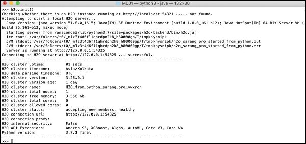
>>>h2o.init()

Your screen would show the cluster information and should look the following at this stage −

Now, you are ready to run the sample code. Type the following command on the Python prompt and execute it.

>>>h2o.demo("glm")

The demo consists of a Python notebook with a series of commands. After executing each command, its output is shown immediately on the screen and you will be asked to hit the key to continue with the next step. The partial screenshot on executing the last statement in the notebook is shown here −

At this stage your Python installation is complete and you are ready for your own experimentation.

Install in R

Installing H2O for R development is very much similar to installing it for Python, except that you would be using R prompt for the installation.

Starting R Console

Start R console by clicking on the R application icon on your machine. The console screen would appear as shown in the following screenshot −

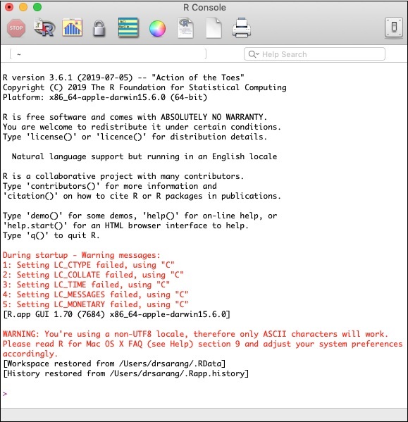
Your H2O installation would be done on the above R prompt. If you prefer using RStudio, type the commands in the R console subwindow.

Removing Older Versions

To begin with, remove older versions using the following command on the R prompt −

> if ("package:h2o" %in% search()) { detach("package:h2o", unload=TRUE) }
> if ("h2o" %in% rownames(installed.packages())) { remove.packages("h2o") }

Downloading Dependencies

Download the dependencies for H2O using the following code −

> pkgs <- c("RCurl","jsonlite")
for (pkg in pkgs) {
   if (! (pkg %in% rownames(installed.packages()))) { install.packages(pkg) }
}

Installing H2O

Install H2O by typing the following command on the R prompt −

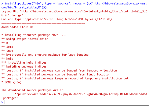
> install.packages("h2o", type = "source", repos = (c("http://h2o-release.s3.amazonaws.com/h2o/latest_stable_R")))

The following screenshot shows the expected output −

There is another way of installing H2O in R.

Install in R from CRAN

To install R from CRAN, use the following command on R prompt −

> install.packages("h2o")

You will be asked to select the mirror −

--- Please select a CRAN mirror for use in this session ---

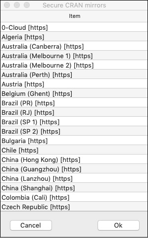
A dialog box displaying the list of mirror sites is shown on your screen. Select the nearest location or the mirror of your choice.

Testing Installation

On the R prompt, type and run the following code −

> library(h2o)
> localH2O = h2o.init()
> demo(h2o.kmeans)

The output generated will be as shown in the following screenshot −

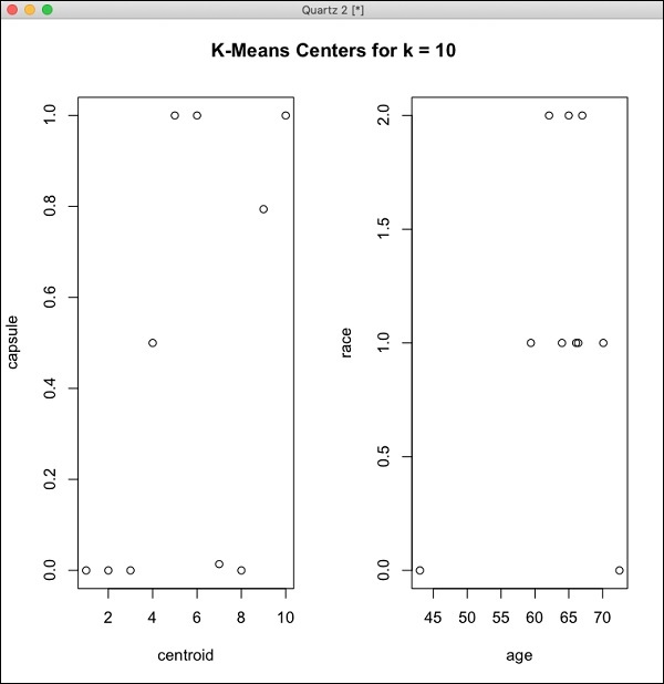
Your H2O installation in R is complete now.

Installing Web GUI Flow

To install GUI Flow download the installation file from the H20 site. Unzip the downloaded file in your preferred folder. Note the presence of h2o.jar file in the installation. Run this file in a command window using the following command −

$ java -jar h2o.jar

After a while, the following will appear in your console window.

07-24 16:06:37.304 192.168.1.18:54321 3294 main INFO: H2O started in 7725ms
07-24 16:06:37.304 192.168.1.18:54321 3294 main INFO:
07-24 16:06:37.305 192.168.1.18:54321 3294 main INFO: Open H2O Flow in your web browser: http://192.168.1.18:54321
07-24 16:06:37.305 192.168.1.18:54321 3294 main INFO:

To start the Flow, open the given URL http://localhost:54321 in your browser. The following screen will appear −

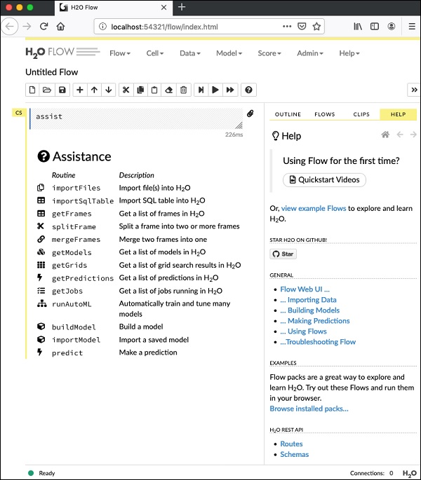
At this stage, your Flow installation is complete.

Install on Hadoop / Anaconda Cloud

Unless you are a seasoned developer, you would not think of using H2O on Big Data. It is sufficient to say here that H2O models run efficiently on huge databases of several terabytes. If your data is on your Hadoop installation or in the Cloud, follow the steps given on H2O site to install it for your respective database.

Now that you have successfully installed and tested H2O on your machine, you are ready for real development. First, we will see the development from a Command prompt. In our subsequent lessons, we will learn how to do model testing in H2O Flow.

Developing in Command Prompt

Let us now consider using H2O to classify plants of the well-known iris dataset that is freely available for developing Machine Learning applications.

Start the Python interpreter by typing the following command in your shell window −

$ Python3

This starts the Python interpreter. Import h2o platform using the following command −

>>> import h2o

We will use Random Forest algorithm for classification. This is provided in the H2ORandomForestEstimator package. We import this package using the import statement as follows −

>>> from h2o.estimators import H2ORandomForestEstimator

We initialize the H2o environment by calling its init method.

>>> h2o.init()

On successful initialization, you should see the following message on the console along with the cluster information.

Checking whether there is an H2O instance running at http://localhost:54321 . connected.

Now, we will import the iris data using the import_file method in H2O.

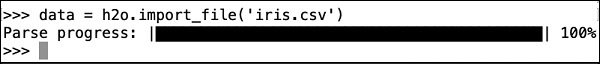
>>> data = h2o.import_file('iris.csv')

The progress will display as shown in the following screenshot −

After the file is loaded in the memory, you can verify this by displaying the first 10 rows of the loaded table. You use the head method to do so −

>>> data.head()

You will see the following output in tabular format.

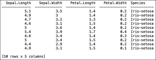
The table also displays the column names. We will use the first four columns as the features for our ML algorithm and the last column class as the predicted output. We specify this in the call to our ML algorithm by first creating the following two variables.

>>> features = ['sepal_length', 'sepal_width', 'petal_length', 'petal_width']
>>> output = 'class'

Next, we split the data into training and testing by calling the split_frame method.

>>> train, test = data.split_frame(ratios = [0.8])

The data is split in the 80:20 ratio. We use 80% data for training and 20% for testing.

Now, we load the built-in Random Forest model into the system.

>>> model = H2ORandomForestEstimator(ntrees = 50, max_depth = 20, nfolds = 10)

In the above call, we set the number of trees to 50, the maximum depth for the tree to 20 and number of folds for cross validation to 10. We now need to train the model. We do so by calling the train method as follows −

>>> model.train(x = features, y = output, training_frame = train)

The train method receives the features and the output that we created earlier as first two parameters. The training dataset is set to train, which is the 80% of our full dataset. During training, you will see the progress as shown here −

Now, as the model building process is over, it is time to test the model. We do this by calling the model_performance method on the trained model object.

>>> performance = model.model_performance(test_data=test)

In the above method call, we sent test data as our parameter.

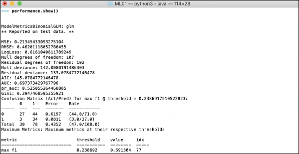
It is time now to see the output, which is the performance of our model. You do this by simply printing the performance.

>>> print (performance)

This will give you the following output −

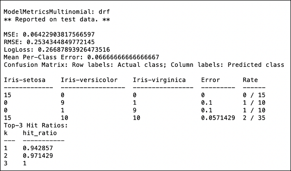
The output shows the Mean Square Error (MSE), Root Mean Square Error (RMSE), LogLoss and even the Confusion Matrix.

Running in Jupyter

We have seen the execution from the command and also understood the purpose of each line of code. You may run the entire code in a Jupyter environment, either line by line or the whole program at a time. The complete listing is given here −

import h2o
from h2o.estimators import H2ORandomForestEstimator
h2o.init()
data = h2o.import_file('iris.csv')
features = ['sepal_length', 'sepal_width', 'petal_length', 'petal_width']
output = 'class'
train, test = data.split_frame(ratios=[0.8])
model = H2ORandomForestEstimator(ntrees = 50, max_depth = 20, nfolds = 10)
model.train(x = features, y = output, training_frame = train)
performance = model.model_performance(test_data=test)
print (performance)

Run the code and observe the output. You can now appreciate how easy it is to apply and test a Random Forest algorithm on your dataset. The power of H20 goes far beyond this capability. What if you want to try another model on the same dataset to see if you can get better performance. This is explained in our subsequent section.

Applying a Different Algorithm

Now, we will learn how to apply a Gradient Boosting algorithm to our earlier dataset to see how it performs. In the above full listing, you will need to make only two minor changes as highlighted in the code below −

import h2o 
from h2o.estimators import H2OGradientBoostingEstimator
h2o.init()
data = h2o.import_file('iris.csv')
features = ['sepal_length', 'sepal_width', 'petal_length', 'petal_width']
output = 'class'
train, test = data.split_frame(ratios = [0.8]) 
model = H2OGradientBoostingEstimator
(ntrees = 50, max_depth = 20, nfolds = 10)
model.train(x = features, y = output, training_frame = train)
performance = model.model_performance(test_data = test)
print (performance)

Run the code and you will get the following output −

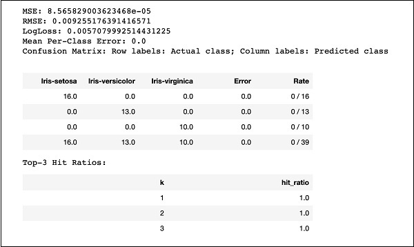
Just compare the results like MSE, RMSE, Confusion Matrix, etc. with the previous output and decide on which one to use for production deployment. As a matter of fact, you can apply several different algorithms to decide on the best one that meets your purpose.