- Generative AI - Home
- Generative AI Basics
- Generative AI Basics
- Generative AI Evolution
- ML and Generative AI
- Generative AI Models
- Discriminative vs Generative Models
- Types of Gen AI Models
- Probability Distribution
- Probability Density Functions
- Maximum Likelihood Estimation
- Generative AI Networks
- How GANs Work?
- GAN - Architecture
- Conditional GANs
- StyleGAN and CycleGAN
- Training a GAN
- GAN Applications
- Generative AI Transformer
- Transformers in Gen AI
- Architecture of Transformers in Gen AI
- Input Embeddings in Transformers
- Multi-Head Attention
- Positional Encoding
- Feed Forward Neural Network
- Residual Connections in Transformers
- Generative AI Autoencoders
- Autoencoders in Gen AI
- Autoencoders Types and Applications
- Implement Autoencoders Using Python
- Variational Autoencoders
- Generative AI and ChatGPT
- A Generative AI Model
- Generative AI Miscellaneous
- Gen AI for Manufacturing
- Gen AI for Developers
- Gen AI for Cybersecurity
- Gen AI for Software Testing
- Gen AI for Marketing
- Gen AI for Educators
- Gen AI for Healthcare
- Gen AI for Students
- Gen AI for Industry
- Gen AI for Movies
- Gen AI for Music
- Gen AI for Cooking
- Gen AI for Media
- Gen AI for Communications
- Gen AI for Photography
Training a Generative Adversarial Network (GANs)
We explored the architecture of Generative Adversarial Networks and how they work. In this chapter, we will take a practical example to demonstrate how you can implement and train a GAN to generate handwritten digits, same as those in the MNIST dataset. We'll use Python along with TensorFlow and Keras for this example.
Process of Training a Generative Adversarial Network
The training of GANs involves optimizing both the generator model and the discriminator model iteratively. Lets understand the training process of a Generative Adversarial Network (GAN) using the following steps:
Initialization
- The process starts with two neural networks: the Generator Network (G) and the Discriminator Network (D).
- The Generator takes a random seed or noise vector as input and produces generated samples.
- The Discriminator takes either real data samples or generated samples as input and classifies them as real or fake.
Generating Fake Data
- A random noise vector is fed into the Generator Network.
- The Generator processes this noise and outputs generated data samples that are intended to resemble real data.
Generator Training
- First it generates fake data from input random noise.
- Then it calculates the generators loss using the discriminators output.
- Finally, it updates the generators weights to minimize the loss.
Discriminator Training
- First, it takes a batch of real data and a batch of fake data.
- Then it calculates the discriminators loss for both real and fake data.
- Finally, it updates the discriminators weights to minimize the loss.
Iterative Training
- Repeat steps 2 to 4. During each iteration, both the Generator and Discriminator are alternately trained and try to improve each other's performance.
- This alternating optimization continues until the generator generates data that is identical to the real data and the discriminator can no longer reliably distinguish between real and fake data.
Training and Building a GAN
Here, we will show the step-by-step procedure of training and building a GAN using Python and the MNIST dataset −
Step 1: Setting Up the Environment
Before we start, we need to set up our Python environment with the necessary libraries. Ensure you have TensorFlow and Keras installed on your computer. You can install them using pip as follows −
pip install tensorflow
Step 2: Import Necessary Libraries
We need to import the essential libraries −
import numpy as np
import tensorflow as tf
from tensorflow.keras import layers, models
from tensorflow.keras.datasets import mnist
import matplotlib.pyplot as plt
Step 3: Load and Preprocess the MNIST Dataset
The MNIST dataset consists of 60,000 training images and 10,000 testing images of handwritten digits, each of size 28x28 pixels. We will normalize the pixel values to the range [-1, 1] to make training more efficient −
# Load the dataset
(x_train, _), (_, _) = mnist.load_data()

# Normalize the images to [-1, 1]
x_train = (x_train - 127.5) / 127.5
x_train = np.expand_dims(x_train, axis=-1)

# Set batch size and buffer size
BUFFER_SIZE = 60000
BATCH_SIZE = 256
Step 4: Create the Generator and Discriminator Models
The generator creates fake images from random noise, and the discriminator attempts to distinguish between real and fake images.
Implementation the Generator Model
The generator model takes a random noise vector as input and transforms it through a series of layers to produce a fake image −
def build_generator():
   model = models.Sequential()
   model.add(layers.Dense(256, use_bias=False, input_shape=(100,)))
   model.add(layers.BatchNormalization())
   model.add(layers.LeakyReLU())

   model.add(layers.Dense(512, use_bias=False))
   model.add(layers.BatchNormalization())
   model.add(layers.LeakyReLU())

   model.add(layers.Dense(28 * 28 * 1, use_bias=False, activation='tanh'))
   model.add(layers.Reshape((28, 28, 1)))

   return model

generator = build_generator()
Implementation the Discriminator Model
The discriminator model takes an image as input (either real or generated) and outputs a probability value indicating whether the image is real or fake −
def build_discriminator():
   model = models.Sequential()
   model.add(layers.Flatten(input_shape=(28, 28, 1)))
   model.add(layers.Dense(512))
   model.add(layers.LeakyReLU())
   model.add(layers.Dropout(0.3))

   model.add(layers.Dense(256))
   model.add(layers.LeakyReLU())
   model.add(layers.Dropout(0.3))

   model.add(layers.Dense(1, activation='sigmoid'))

   return model

discriminator = build_discriminator()
Step 5: Define Loss Functions and Optimizers
In this step, we will use binary cross-entropy loss for both the generator and discriminator. The generator aims to maximize the probability of the discriminator making a mistake, while the discriminator aims to minimize its classification error.
cross_entropy = tf.keras.losses.BinaryCrossentropy(from_logits=True)

def generator_loss(fake_output):
   return cross_entropy(tf.ones_like(fake_output), fake_output)

def discriminator_loss(real_output, fake_output):
   real_loss = cross_entropy(tf.ones_like(real_output), real_output)
   fake_loss = cross_entropy(tf.zeros_like(fake_output), fake_output)
   total_loss = real_loss + fake_loss
   return total_loss

generator_optimizer = tf.keras.optimizers.Adam(1e-4)
discriminator_optimizer = tf.keras.optimizers.Adam(1e-4)
Step 6: Define the Training Loop
The training process for a GAN involves training the generator and discriminator iteratively. Here, we will define a training step that includes generating fake images, calculating losses, and updating the model weights using backpropagation.
@tf.function
def train_step(images):
   noise = tf.random.normal([BATCH_SIZE, 100])

   with tf.GradientTape() as gen_tape, tf.GradientTape() as disc_tape:
      generated_images = generator(noise, training=True)

      real_output = discriminator(images, training=True)
      fake_output = discriminator(generated_images, training=True)

      gen_loss = generator_loss(fake_output)
      disc_loss = discriminator_loss(real_output, fake_output)

   gradients_of_generator = gen_tape.gradient(gen_loss, generator.trainable_variables)
   gradients_of_discriminator = disc_tape.gradient(disc_loss, discriminator.trainable_variables)

   generator_optimizer.apply_gradients(zip(gradients_of_generator, generator.trainable_variables))
   discriminator_optimizer.apply_gradients(zip(gradients_of_discriminator, discriminator.trainable_variables))

def train(dataset, epochs):
   for epoch in range(epochs):
      for image_batch in dataset:
         train_step(image_batch)
      print(f'Epoch {epoch+1} completed')
Step 7: Prepare the Dataset and Train the GAN
Next, we will prepare the dataset by shuffling and batching the MNIST images and then we will start the training process.
# Prepare the dataset for training
train_dataset = tf.data.Dataset.from_tensor_slices(x_train).shuffle(BUFFER_SIZE).batch(BATCH_SIZE)

# Train the GAN
EPOCHS = 50
train(train_dataset, EPOCHS)
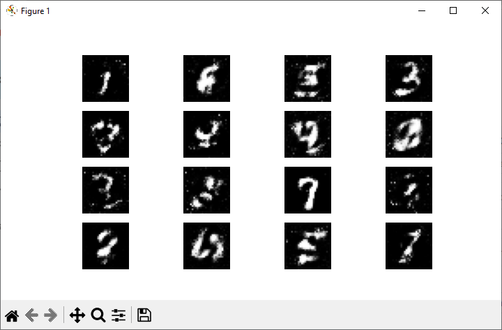
Step 8: Generate and Display Images
Now, after training the GAN, we can generate and display new images created by the generator. It involves creating random noise, feeding it to the generator, and displaying the resulting images.
def generate_and_save_images(model, epoch, test_input):
   predictions = model(test_input, training=False)

   fig = plt.figure(figsize=(7.50, 3.50))

   for i in range(predictions.shape[0]):
      plt.subplot(4, 4, i + 1)
      plt.imshow(predictions[i, :, :, 0] * 127.5 + 127.5, cmap='gray')
      plt.axis('off')

   plt.savefig('image_at_epoch_{:04d}.png'.format(epoch))
   plt.show()

seed = tf.random.normal([16, 100])
generate_and_save_images(generator, EPOCHS, seed)
After implementation, when you run this code, you will get the following output −
Conclusion
Training a GAN using Python involves several key steps such as setting up the environment, creating the generator and discriminator models, defining loss functions and optimizers, and implementing the training loop. By following these steps, you can train your own GAN and explore the fascinating world of generative adversarial networks.
In this chapter, we provided a detailed guide to building and training a GAN using Python programming language. We used TensorFlow and Keras libraries and the MNIST dataset for our example.