- Excel Pivot Tables - Home
- Excel Pivot Tables - Overview
- Excel Pivot Tables - Creation
- Excel Pivot Tables - Fields
- Excel Pivot Tables - Areas
- Excel Pivot Tables - Exploring Data
- Excel Pivot Tables - Sorting Data
- Excel Pivot Tables - Filtering Data
- Filtering data using Slicers
- Excel Pivot Tables - Nesting
- Excel Pivot Tables - Tools
- Summarizing Values
- Excel Pivot Tables - Updating Data
- Excel Pivot Tables - Reports
Excel Pivot Tables - Summarizing Values
You can summarize a PivotTable by placing a field in ∑ VALUES area in the PivotTable Fields Task pane. By default, Excel takes the summarization as sum of the values of the field in ∑ VALUES area. However, you have other calculation types, such as, Count, Average, Max, Min, etc.
In this chapter, you will learn how to set a calculation type based on how you want to summarize the data in the PivotTable.
Sum
Consider the following PivotTable wherein you have the summarized sales data regionwise, salesperson-wise and month-wise.
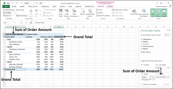
As you can observe, when you drag the field Order Amount to ∑ VALUES area, it is displayed as Sum of Order Amount, indicating the calculation is taken as Sum. In the PivotTable, in the top-left corner, Sum of Order Amount is displayed. Further, Grand Total column and Grand Total row are displayed for subtotals field-wise in rows and columns respectively.
Value Field Settings
With Values Field Settings, you can set the calculation type in your PivotTable. You can also decide on how you want to display your values.
- Click on Sum of Order Amount in ∑ VALUES area.
- Select Value Field Settings from the dropdown list.
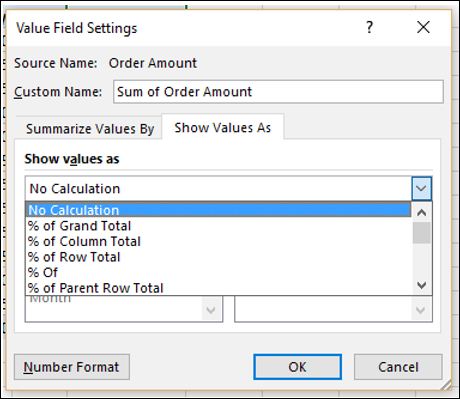
The Value Field Settings dialog box appears.
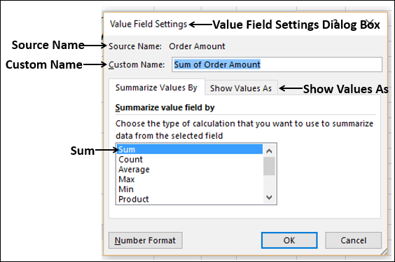
The Source Name is the field and Custom Name is Sum of field. Calculation Type is Sum. Click the Show Values As tab.
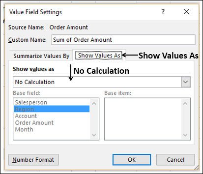
In the box Show Values As, No Calculation is displayed. Click the Show Values As box. You can find several ways of showing your total values.
% of Grand Total
You can show the values in the PivotTable as % of Grand Total.
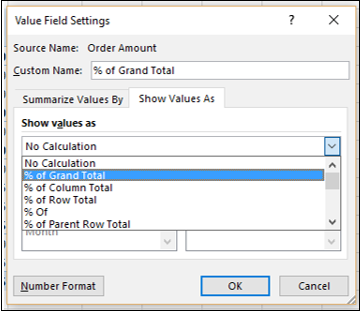
- In the Custom Name box, type % of Grand Total.
- Click on the Show Values As box.
- Click on % of Grand Total in the dropdown list. Click OK.
The PivotTable summarizes the values as % of the Grand Total.
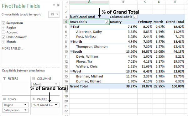
As you can observe, Sum of Order Amount in the top-left corner of the PivotTable and in the ∑ VALUES area in the PivotTable Fields pane is changed to the new Custom Name - % of Grand Total.
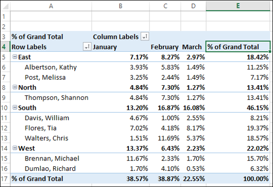
Click on the header of the Grand Total column.
Type % of Grand Total in the formula bar. Both the Column and Row headers will change to % of Grand Total.
% of Column Total
Suppose you want to summarize the values as % of each month total.
Click on Sum of Order Amount in ∑ VALUES area.
Select Value Field Settings from the dropdown list. The Value Field Settings dialog box appears.
In the Custom Name box, type % of Month Total.
Click on the Show values as box.
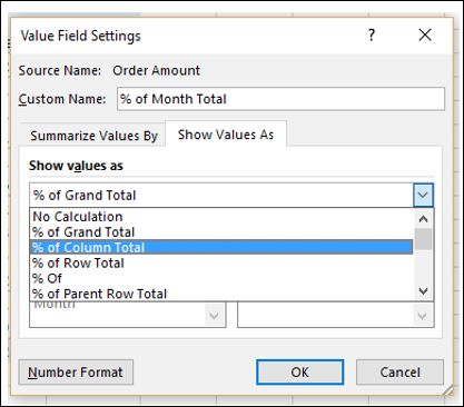
Select % of Column Total from the dropdown list.
Click OK.
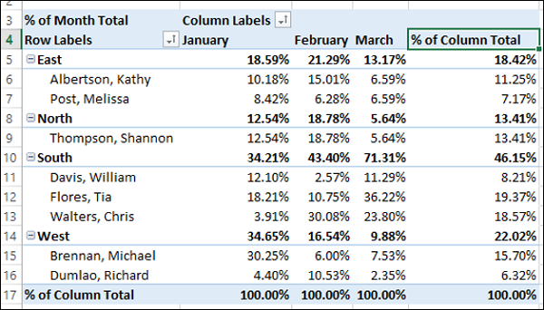
The PivotTable summarizes the values as % of the Column Total. In the Month columns, you will find the values as % of the specific month total.
Click on the header of the Grand Total column.
Type % of Column Total in the formula bar. Both the Column and Row headers will change to % of Column Total.
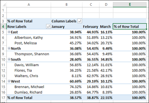
% of Row Total
You can summarize the values as % of region totals and % of salesperson totals, by selecting % of Row Total in Show Values As box in the Value Field Settings dialog box.
Count
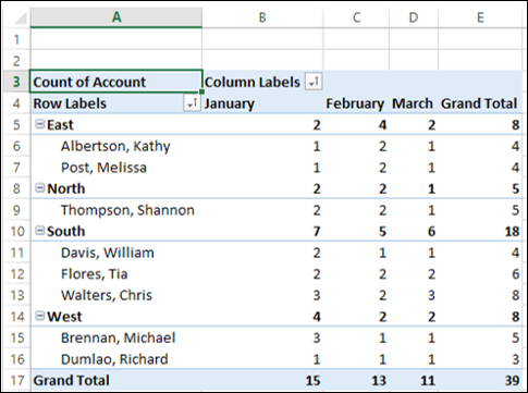
Suppose you want to summarize the values by the number of Accounts region wise, salesperson wise and month wise.
Deselect Order Amount.
Drag Account to ∑ VALUES area. The Sum of Account will be displayed in the ∑ VALUES area.
Click on Sum of Account.
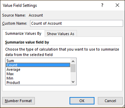
Select Value Field Settings from the dropdown list. The Value Field Settings dialog box appears.
In the Summarize value field by box, select Count. The Custom Name changes to Count of Account.
Click OK.
The Count of Account will be displayed as shown below −
Average
Suppose you want to summarize the PivotTable by average values of Order Amount region wise, salesperson wise and month wise.
Deselect Account.
Drag Order Amount to ∑ VALUES area. The Sum of Order Amount will be displayed in the ∑ VALUES area.
Click on Sum of Order Amount.
Click on Value Field Settings in the dropdown list. The Value Field Settings dialog box appears.
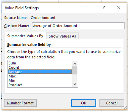
In the Summarize value field by box, click on Average. The Custom Name changes to Average of Order Amount.
Click OK.
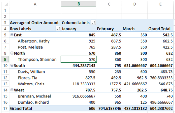
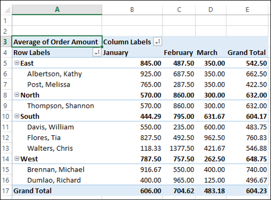
The average will be displayed as shown below −
You have to set the number format of the values in the PivotTable to make it more presentable.
Click on Average of Order Amount in ∑ VALUES area.
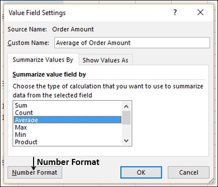
Click on Value Field Settings in the dropdown list. The Value Field Settings dialog box appears.
Click on the Number Format button.
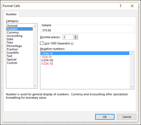
The Format Cells dialog box appears.
- Click on Number under Category.
- Type 2 in the Decimal places box and click OK.
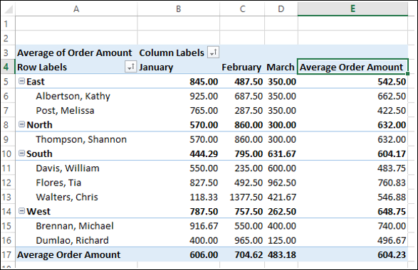
The PivotTable values will be formatted to numbers with two decimal places.
Click on the header of the Grand Total column.
Type Average Order Amount in the formula bar. Both the Column and Row headers will change to Average Order Amount.
Max
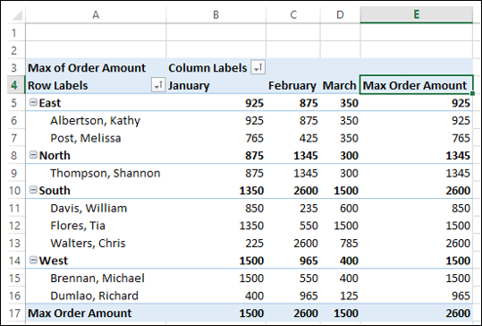
Suppose you want to summarize the PivotTable by the maximum values of Order Amount region-wise, salesperson-wise and month-wise.
Click on Sum of Order Amount.
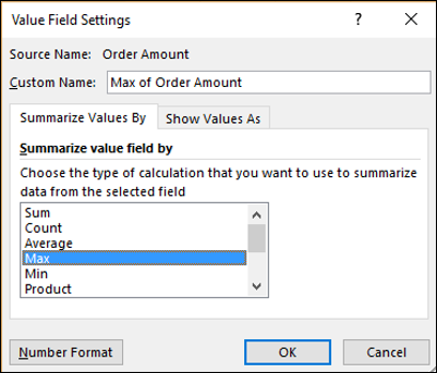
Select Value Field Settings from the dropdown list. The Value Field Settings dialog box appears.
In the Summarize value field by box, click Max. The Custom Name changes to Max of Order Amount.
The PivotTable will display the maximum values region wise, salesperson wise and month wise.
Click on the header the Grand Total column.
Type Max Order Amount in the formula bar. Both the Column and Row headers will change to Max Order Amount.
Min
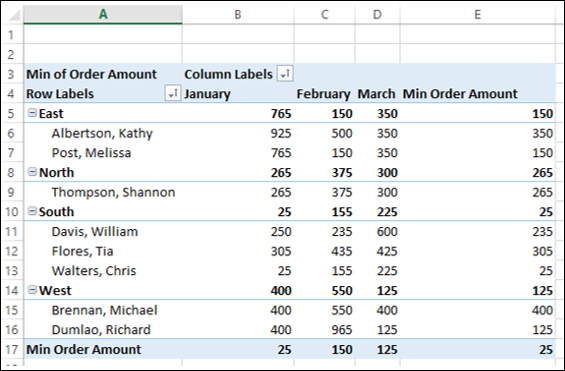
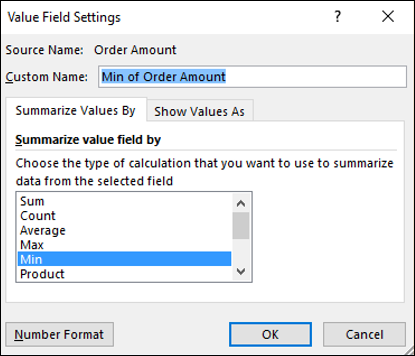
Suppose you want to summarize the PivotTable by the minimum values of Order Amount region wise, salesperson wise and month wise.
Click on Sum of Order Amount.
Click on Value Field Settings in the dropdown list. The Value Field Settings dialog box appears.
In the Summarize value field by box, click Min. The Custom Name changes to Min of Order Amount.
The PivotTable will display the minimum values region wise, salesperson wise and month wise.
Click on the header of the Grand Total column.
Type Min Order Amount in the formula bar. Both the Column and Row headers will change to Min Order Amount.