- Excel Pivot Tables - Home
- Excel Pivot Tables - Overview
- Excel Pivot Tables - Creation
- Excel Pivot Tables - Fields
- Excel Pivot Tables - Areas
- Excel Pivot Tables - Exploring Data
- Excel Pivot Tables - Sorting Data
- Excel Pivot Tables - Filtering Data
- Filtering data using Slicers
- Excel Pivot Tables - Nesting
- Excel Pivot Tables - Tools
- Summarizing Values
- Excel Pivot Tables - Updating Data
- Excel Pivot Tables - Reports
Excel Pivot Tables - Areas
PivotTable areas are a part of PivotTable Fields Task Pane. By arranging the selected fields in the areas, you can arrive at different PivotTable layouts. As you can simply drag the fields across areas, you can quickly switch across the different layouts, summarizing the data, in a way you want.
You have already learnt about PivotTable Fields Task Pane in the earlier chapter on PivotTable Fields in this tutorial. In this chapter, you will learn about the PivotTable areas.
There are four PivotTable areas available −
- ROWS.
- COLUMNS.
- FILTERS.
- ∑ VALUES (Read as Summarizing Values).
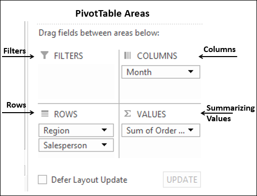
The message - Drag fields between areas below appears above the areas.
With PivotTable Areas, you can choose −
- What fields to display as rows (ROWS area).
- What fields to display as columns (COLUMNS area).
- How to summarize your data (∑ VALUES area).
- Filters for any of the fields (FILTERS area).
You can just drag the fields across these areas and observe how the PivotTable Layout changes.
ROWS
If you select the fields in the PivotTable Fields lists by just checking the boxes, all the nonnumeric fields will automatically be added to the ROWS area, in the order you select.
You can optionally, drag a field to the ROWS area. The fields that are put in ROWS area appear as rows in the PivotTable, with the Row Labels being the values of the selected fields.
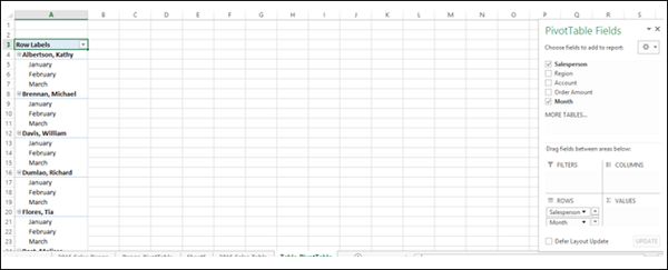
For example, consider the Sales data table.
- Drag the field Salesperson to ROWS area.
- Drag the field Month to ROWS area.
Your PivotTable appears with one column containing the Row Labels Salesperson and Month and a last row as Grand Total, as given below.
COLUMNS
You can drag fields to the COLUMNS area.
The fields that are put in COLUMNS area appear as columns in the PivotTable, with the Column Labels being the values of the selected fields.
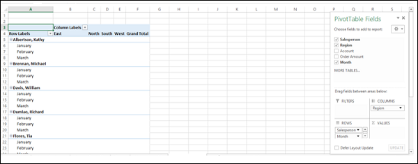
Drag the field Region to COLUMNS area. Your PivotTable appears with the first column containing the Row Labels Salesperson and Month the next four columns containing the Column Labels Region and a last column Grand Total as given below.
Drag the field Month from ROWS to COLUMNS.
Drag the field Region from COLUMNS to ROWS. Your PivotTable layout changes as given below.
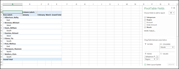
You can see that there are only five columns now the first column with Row Labels, three columns with Column Labels and a last column with Grand Total.
The number of Rows and Columns is based on the number of values you have in those fields.
∑ VALUES
The primary use of a PivotTable is to summarize values. Hence, by placing the fields by which you want to summarize the data in ∑ VALUES area, you arrive at the summary table.
Drag the field Order Amount to ∑ VALUES.
Drag the field Region to above the field Salesperson in ROWS area. This step is to change the nesting order. You will learn nesting in the chapter Nesting in the PivotTable in this tutorial.
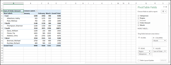
As you can observe, the data is summarized region-wise, salesperson-wise and monthwise. You have subtotals for each region, month wise. You also have grand totals month wise in the Grand Total row grand totals region wise in the Grand Total column.
FILTERS
The Filters area is to place filters in PivotTable. Suppose you want to display results separately for the selected regions only.
Drag the field Region from ROWS area to FILTERS area. The filter Region will be placed above the PivotTable. In case you do not have empty rows above the PivotTable, the PivotTable is pushed down inserting rows above the PivotTable for the filter.
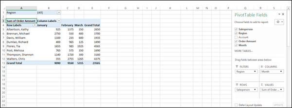
As you can observe, (ALL) appears in the filter by default, and the PivotTable displays data for all the values of the Region.
- Click on the arrow to the right of filter.
- Check the box Select Multiple Items.
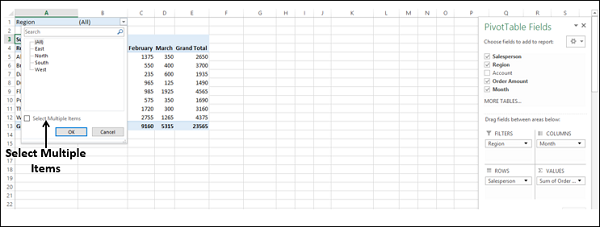
Check boxes will appear for all the options in the dropdown list. By default, all the boxes are checked.
- Check the boxes North and South.
- Clear the other boxes. Click OK.
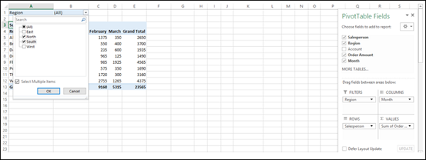
The PivotTable gets changed to reflect the filtered data.
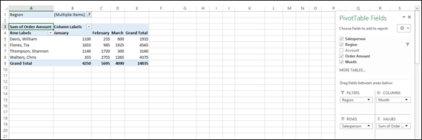
You can observe that the filter displays (Multiple Items). Therefore, when someone is looking at the PivotTable, it is not immediately obvious of what values are filtered.
Excel provides you another tool called Slicers to handle filtering more efficiently. You will understand Filtering Data in a PivotTable in detail in a later chapter in this tutorial.
