Filtering data using Slicers

---

---

Using one or more slicers is a quick and effective way to filter your data. Slicers can be inserted for each of the fields that you want to filter. Slicer will have buttons denoting the values of the field that it represents. You can click on the buttons of a slicer to select/ unselect the values in the field.

Slicers stay visible with the PivotTable and so you will always know what fields are used for filtering and what values in those fields are shown or hidden in the filtered PivotTable.

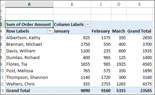
To understand the usage of slicers, consider the example of sales data region-wise, month wise and salesperson-wise. Assume you have the following PivotTable with this data.

Inserting Slicers

Suppose you want to filter this PivotTable based on the fields – Region and Month.

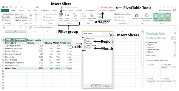
• Click on ANALYZE under PIVOTTABLE TOOLS on the Ribbon.

• Click on Insert Slicer in the Filter group. The Insert Slicers dialog box appears. It contains all the fields from your data table.

• Check the boxes Region and Month.

• Click OK.

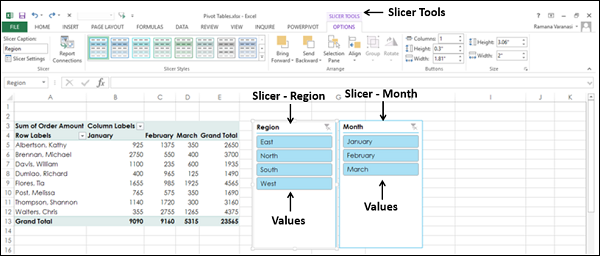
Slicers for each of the selected fields appear with all the values selected by default. Slicer Tools appear on the Ribbon to work on the Slicer settings, look and feel.

Filtering with Slicers

As you can observe, each slicer has all the values of the field that it represents and the values are displayed as buttons. By default, all the values of a field are selected and hence all the buttons are highlighted.

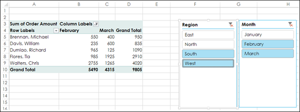
Suppose you want to display the PivotTable only for the regions South and West and for the Months February and March.

• Click on South in the Slicer for Region. Only South will be highlighted in the Slicer – Region.

• Keep Ctrl key pressed and click on West in the Slicer for Region.

• Click on February in the Slicer for Month.

• Keep Ctrl key pressed and click on March in the Slicer for Month.

Selected items in the Slicers are highlighted. PivotTable with summarized values for the selected items will be displayed.

To add/remove values of a field from the filter, keep the Ctrl key pressed and click on those buttons in the slicer of the field.

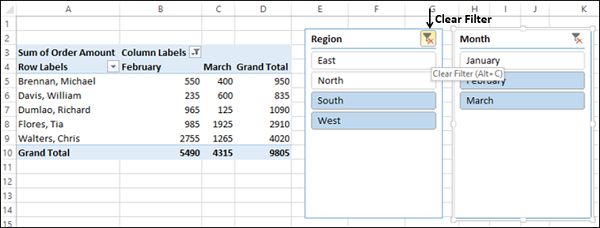
Clearing the Filter in a Slicer

To clear the filter in a slicer, click on at the top-right corner of the slicer.

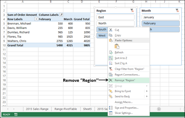
Removing a Slicer

Suppose you want to remove the slicer for the Region field.

• Right click on the Slicer – Region.
• Click on Remove “Region” in the dropdown list.

Slicer Tools

Once you insert a slicer, Slicer Tools appear on the Ribbon with OPTIONS tab. To view Slicer Tools, click on a slicer.

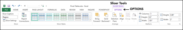
As you can observe, under the Slicer Tools – OPTION tab, you have several options to change the look and feel of the slicer that include −

• Slicer Caption
• Slicer Settings
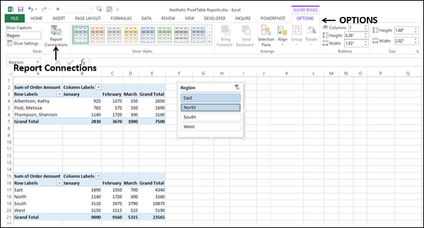
• Report Connections
• Selection Pane

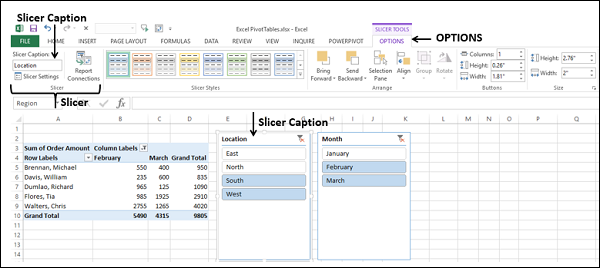
Slicer Caption

You can find the Slicer Caption box in the Slicer group. The Slicer Caption is the header that is displayed on the slicer. By default, Slicer Caption is the name of the field that it represents.

• Click on the Slicer for Region.
• Click the OPTIONS tab on the Ribbon.

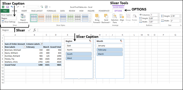
The Slicer group on the Ribbon, in the Slicer Caption box, Region is displayed as the header of the slicer. It is the name of the field for which the slicer is inserted. You can change the Slicer Caption as follows −

• Click on the Slicer Caption box in the Slicer group on the Ribbon.

• Delete Region. The box is cleared.

• Type Location in the box and press Enter. The Slicer Caption changes to Location and the same is reflected as header in the slicer.

Note − You have changed only the slicer caption, i.e. the header. The name of the field that the slicer represents – Region remains as it is.

Slicer Settings

You can use Slicer Settings to change the name of the slicer, change the slicer caption, choose whether to display the slicer header or not and set the sorting and filtering options for the items −

• Click on the slicer - Location.

• Click the OPTIONS tab on the Ribbon. You can find the Slicer Settings in the Slicer group on the Ribbon. You can also find Slicer Settings in the dropdown list when you right click on the slicer.

• Click the Slicer Settings. The Slicer Settings dialog box appears.

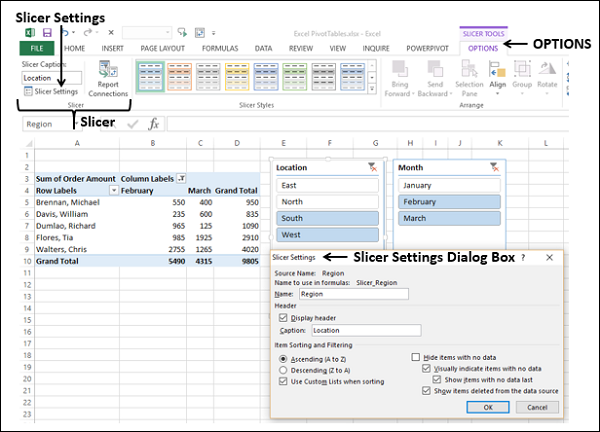
As you can observe, the following are fixed for the slicer −

• Source Name.
• Name to use in formulas.

You can change the following for the slicer −

• Name.
• Header – Caption.
• Display header.
• Sorting and Filtering options for the items displayed on the slicer.

Report Connections

You can connect different PivotTables to a Slicer, provided one of the following holds good −

• The PivotTables are created using the same data.

• One PivotTable has been copied and pasted as an additional PivotTable.

• Multiple PivotTables are created on separate sheets with Show Report Filter Pages.

Consider the following PivotTables that are created from the same data −

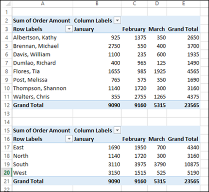
• Name the top PivotTable as PivotTable-Top and the bottom one as PivotTable-Bottom.
• Click on the top PivotTable.
• Insert a Slicer for the field Region.
• Select East and North on the Slicer.

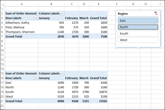
Observe that the filtering is applied only to the top PivotTable and not to the bottom PivotTable. You can use the same slicer for both the PivotTables by connecting it to the bottom PivotTable also as follows −

• Click on the slicer - Region. The SLICER TOOLS appear on the Ribbon.
• Click the OPTIONS tab on the Ribbon.

You will find Report Connections in the Slicer group on the Ribbon. You can also find Report Connections in the dropdown list when you right click on the slicer.

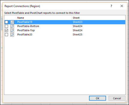
Click Report Connections in the Slicer group.

The Report Connections dialog box appears. The box PivotTable-Top is checked and other boxes are unchecked. Check the box PivotTable-Bottom also and click OK.

The bottom PivotTable will be filtered to the selected items – East and North.

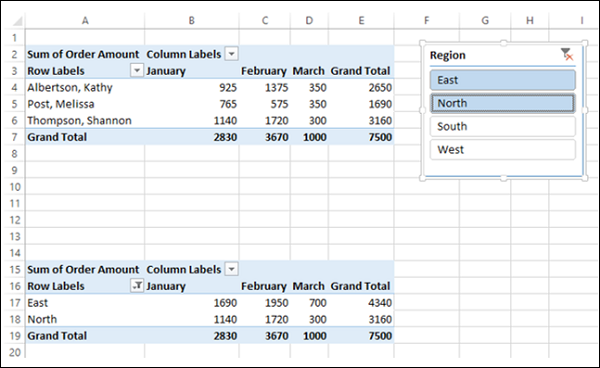
This became possible because both the PivotTables are now connected to the slicer. If you make changes in the selections in the slicer, the same filtering will appear in both the PivotTables.

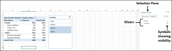
Selection Pane

You can switch the display of the slicers on the worksheet off and on using the Selection Pane.

• Click on the slicer - Location.

• Click the OPTIONS tab on the Ribbon.

• Click the Selection Pane in the Arrange group on the Ribbon. The Selection Pane appears on the right side of the window.

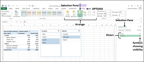
As you can observe, the names of all the slicers are listed in the Selection pane. On the right side of the names, you can find the visibility symbol - indicating the slicer is visible on the worksheet.

Click the symbol for Month. The symbol changes to the symbol , indicating that the slicer is hidden (not visible).

As you can observe, the slicer – Month is not shown on the worksheet. However, remember that you did not remove the slicer for Month, but you have just hidden it.

• Click on the symbol for Month.

• The symbol changes to the symbol , indicating that the slicer is now visible.

When you switch the visibility of a slicer on / off, the selection of the items in that slicer for filtering remain unaltered. You can also change the order of the slicers in the Selection pane by dragging them up/down.