
Article Categories
- All Categories
-
 Data Structure
-
 Networking
-
 RDBMS
RDBMS
-
 Operating System
-
 Java
Java
-
 MS Excel
-
 iOS
iOS
-
 HTML
HTML
-
 CSS
CSS
-
 Android
-
 Python
-
 C Programming
-
 C++
C++
-
 C#
C#
-
 MongoDB
-
 MySQL
MySQL
-
 Javascript
-
 PHP
PHP
Digital Band Pass Butterworth Filter in Python
A Band pass filter is the filter which passes the frequencies within the given range of frequencies and rejects the frequencies which are outside the defined range. The Butterworth band pass filter designed to have the frequency response flat as much as possible to be in the pass band. The following are the specifications of the digital band pass butter worth filter.
The sampling rate of the filter is around 40 kHz.
The pass band edge frequencies are in the range of 1400 Hz to 2100 Hz.
The stop band edge frequencies are within the range of 1050 Hz to 2450 Hz.
The ripple point of the pass band is 0.4 decibels.
The minimum attenuation of the stop band is 50 decibels.
Implementing digital band pass Butterworth filter
To implement the digital band, pass butter worth filter there is a step by step approach. Let?s see each step in detail.
Step 1 First we have to define the sampling frequency fs our input signal, lower cutoff frequency f1, upper cutoff frequency f2 and the order of the filter. If we determine the higher order of the filter, it will result in steeper roll-off which causes the phase distortion.
Step 2 Next we have to calculate the normalized frequencies of the lower and higher cutoff frequencies f1 and f2 as wn1 and wn2 respectively using the below formula.
$\mathrm{wn = 2 * fn / fs}$
Step 3 After that by using the scipy.signal.butter() function we can design the Butterworth filter of the defined order and normalized frequencies by specifying the btype parameter as band.
Step 4 Now we will apply the filter for the given input signal by using the scipy.signal.filtfilt() function to perform zero phase filtering.
Example
In the following example, we are implementing the Digital Band Pass Butterworth filter using the above mentioned steps.
import numpy as np
import matplotlib.pyplot as plt
from scipy.signal import butter, filtfilt
def butter_bandpass(lowcut, highcut, fs, order=5):
nyq = 0.5 * fs
low = lowcut / nyq
high = highcut / nyq
b, a = butter(order, [low, high], btype='band')
return b, a
def butter_bandpass_filter(data, lowcut, highcut, fs, order=5):
b, a = butter_bandpass(lowcut, highcut, fs, order=order)
y = filtfilt(b, a, data)
return y
fs = 1000
t = np.arange(0, 1, 1/fs)
f1 = 10
f2 = 50
sig = np.sin(2*np.pi*f1*t) + np.sin(2*np.pi*f2*t)
order = 4
filtered = butter_bandpass_filter(sig, f1, f2, fs, order)
print("The length of frequencies:",len(filtered))
print("The Butterworth bandpass filter output of first 50 frequencies:",filtered[:50])
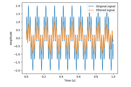
fig, ax = plt.subplots()
ax.plot(t, sig, label='Original signal')
ax.plot(t, filtered, label='Filtered signal')
ax.set_xlabel('Time [s]')
ax.set_ylabel('Amplitude')
ax.legend()
plt.show()
Output
The length of frequencies: 1000
The Butterworth bandpass filter output of first 50 frequencies: [-0.11133763  0.06408296  0.22202113  0.34937958  0.4360314   0.47578308
  0.46696733  0.41260559  0.32012087  0.20062592  0.06785282 -0.0631744
 -0.17759655 -0.26216511 -0.30653645 -0.30428837 -0.2535591  -0.15724548
 -0.02273955  0.13877185  0.31337781  0.48578084  0.64077163  0.76469778
  0.84678346  0.88017133  0.86258464  0.79654483  0.68912261  0.55124662
  0.39663647  0.24046415  0.09787411 -0.01749368 -0.0948334  -0.12722603
 -0.11231195 -0.05251783  0.04518472  0.16996505  0.30819725  0.44479774
  0.5647061   0.65436437  0.70305015  0.70393321  0.65475213  0.5580448
  0.42091007  0.25432388]

2K+ Views
