- Deep Learning with Keras - Home
- Deep Learning with Keras - Introduction
- Deep Learning
- Setting up Project
- Importing Libraries
- Creating Deep Learning Model
- Compiling the Model
- Preparing Data
- Training the Model
- Evaluating Model Performance
- Predicting on Test Data
- Saving Model
- Loading Model for Predictions
- Conclusion
- Deep Learning with Keras Resources
- Deep Learning with Keras - Quick Guide
- Deep Learning with Keras - Useful Resources
- Deep Learning with Keras - Discussion
Deep Learning with Keras - Deep Learning
As said in the introduction, deep learning is a process of training an artificial neural network with a huge amount of data. Once trained, the network will be able to give us the predictions on unseen data. Before I go further in explaining what deep learning is, let us quickly go through some terms used in training a neural network.
Neural Networks
The idea of artificial neural network was derived from neural networks in our brain. A typical neural network consists of three layers input, output and hidden layer as shown in the picture below.
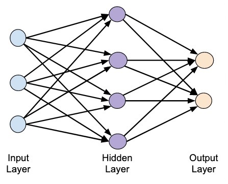
This is also called a shallow neural network, as it contains only one hidden layer. You add more hidden layers in the above architecture to create a more complex architecture.
Deep Networks
The following diagram shows a deep network consisting of four hidden layers, an input layer and an output layer.
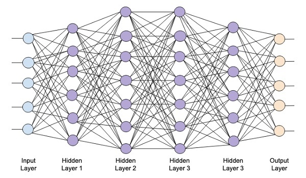
As the number of hidden layers are added to the network, its training becomes more complex in terms of required resources and the time it takes to fully train the network.
Network Training
After you define the network architecture, you train it for doing certain kinds of predictions. Training a network is a process of finding the proper weights for each link in the network. During training, the data flows from Input to Output layers through various hidden layers. As the data always moves in one direction from input to output, we call this network as Feed-forward Network and we call the data propagation as Forward Propagation.
Activation Function
At each layer, we calculate the weighted sum of inputs and feed it to an Activation function. The activation function brings nonlinearity to the network. It is simply some mathematical function that discretizes the output. Some of the most commonly used activations functions are sigmoid, hyperbolic, tangent (tanh), ReLU and Softmax.
Backpropagation
Backpropagation is an algorithm for supervised learning. In Backpropagation, the errors propagate backwards from the output to the input layer. Given an error function, we calculate the gradient of the error function with respect to the weights assigned at each connection. The calculation of the gradient proceeds backwards through the network. The gradient of the final layer of weights is calculated first and the gradient of the first layer of weights is calculated last.
At each layer, the partial computations of the gradient are reused in the computation of the gradient for the previous layer. This is called Gradient Descent.
In this project-based tutorial you will define a feed-forward deep neural network and train it with backpropagation and gradient descent techniques. Luckily, Keras provides us all high level APIs for defining network architecture and training it using gradient descent. Next, you will learn how to do this in Keras.
Handwritten Digit Recognition System
In this mini project, you will apply the techniques described earlier. You will create a deep learning neural network that will be trained for recognizing handwritten digits. In any machine learning project, the first challenge is collecting the data. Especially, for deep learning networks, you need humongous data. Fortunately, for the problem that we are trying to solve, somebody has already created a dataset for training. This is called mnist, which is available as a part of Keras libraries. The dataset consists of several 28x28 pixel images of handwritten digits. You will train your model on the major portion of this dataset and the rest of the data would be used for validating your trained model.
Project Description
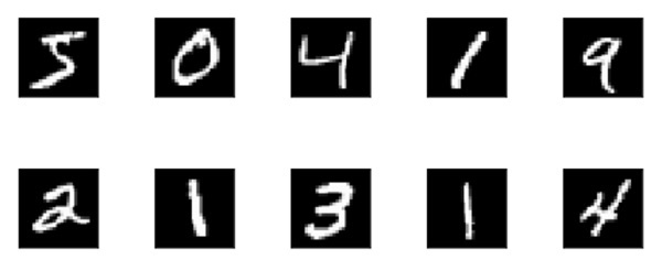
The mnist dataset consists of 70000 images of handwritten digits. A few sample images are reproduced here for your reference
Each image is of size 28 x 28 pixels making it a total of 768 pixels of various gray scale levels. Most of the pixels tend towards black shade while only few of them are towards white. We will put the distribution of these pixels in an array or a vector. For example, the distribution of pixels for a typical image of digits 4 and 5 is shown in the figure below.
Each image is of size 28 x 28 pixels making it a total of 768 pixels of various gray scale levels. Most of the pixels tend towards black shade while only few of them are towards white. We will put the distribution of these pixels in an array or a vector. For example, the distribution of pixels for a typical image of digits 4 and 5 is shown in the figure below.
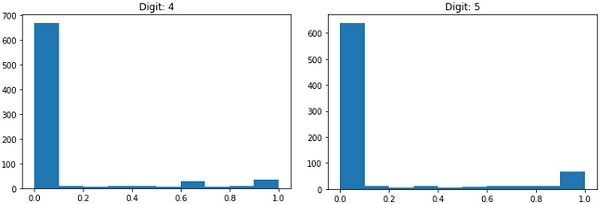
Clearly, you can see that the distribution of the pixels (especially those tending towards white tone) differ, this distinguishes the digits they represent. We will feed this distribution of 784 pixels to our network as its input. The output of the network will consist of 10 categories representing a digit between 0 and 9.
Our network will consist of 4 layers one input layer, one output layer and two hidden layers. Each hidden layer will contain 512 nodes. Each layer is fully connected to the next layer. When we train the network, we will be computing the weights for each connection. We train the network by applying backpropagation and gradient descent that we discussed earlier.
