- Deep Learning with Keras - Home
- Deep Learning with Keras - Introduction
- Deep Learning
- Setting up Project
- Importing Libraries
- Creating Deep Learning Model
- Compiling the Model
- Preparing Data
- Training the Model
- Evaluating Model Performance
- Predicting on Test Data
- Saving Model
- Loading Model for Predictions
- Conclusion
- Deep Learning with Keras Resources
- Deep Learning with Keras - Quick Guide
- Deep Learning with Keras - Useful Resources
- Deep Learning with Keras - Discussion
Evaluating Model Performance
To evaluate the model performance, we call evaluate method as follows −
loss_and_metrics = model.evaluate(X_test, Y_test, verbose=2)
To evaluate the model performance, we call evaluate method as follows −
loss_and_metrics = model.evaluate(X_test, Y_test, verbose=2)
We will print the loss and accuracy using the following two statements −
print("Test Loss", loss_and_metrics[0])
print("Test Accuracy", loss_and_metrics[1])
When you run the above statements, you would see the following output −
Test Loss 0.08041584826191042
Test Accuracy 0.9837
This shows a test accuracy of 98%, which should be acceptable to us. What it means to us that in 2% of the cases, the handwritten digits would not be classified correctly. We will also plot accuracy and loss metrics to see how the model performs on the test data.
Plotting Accuracy Metrics
We use the recorded history during our training to get a plot of accuracy metrics. The following code will plot the accuracy on each epoch. We pick up the training data accuracy (acc) and the validation data accuracy (val_acc) for plotting.
plot.subplot(2,1,1)
plot.plot(history.history['acc'])
plot.plot(history.history['val_acc'])
plot.title('model accuracy')
plot.ylabel('accuracy')
plot.xlabel('epoch')
plot.legend(['train', 'test'], loc='lower right')
The output plot is shown below −
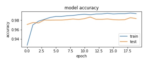
As you can see in the diagram, the accuracy increases rapidly in the first two epochs, indicating that the network is learning fast. Afterwards, the curve flattens indicating that not too many epochs are required to train the model further. Generally, if the training data accuracy (acc) keeps improving while the validation data accuracy (val_acc) gets worse, you are encountering overfitting. It indicates that the model is starting to memorize the data.
We will also plot the loss metrics to check our models performance.
Plotting Loss Metrics
Again, we plot the loss on both the training (loss) and test (val_loss) data. This is done using the following code −
plot.subplot(2,1,2)
plot.plot(history.history['loss'])
plot.plot(history.history['val_loss'])
plot.title('model loss')
plot.ylabel('loss')
plot.xlabel('epoch')
plot.legend(['train', 'test'], loc='upper right')
The output of this code is shown below −
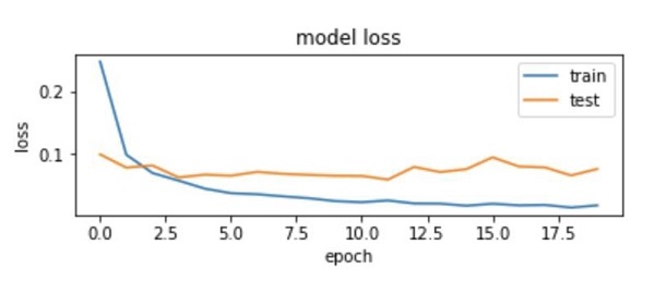
As you can see in the diagram, the loss on the training set decreases rapidly for the first two epochs. For the test set, the loss does not decrease at the same rate as the training set, but remains almost flat for multiple epochs. This means our model is generalizing well to unseen data.
Now, we will use our trained model to predict the digits in our test data.
