- Deep Learning with Keras - Home
- Deep Learning with Keras - Introduction
- Deep Learning
- Setting up Project
- Importing Libraries
- Creating Deep Learning Model
- Compiling the Model
- Preparing Data
- Training the Model
- Evaluating Model Performance
- Predicting on Test Data
- Saving Model
- Loading Model for Predictions
- Conclusion
- Deep Learning with Keras Resources
- Deep Learning with Keras - Quick Guide
- Deep Learning with Keras - Useful Resources
- Deep Learning with Keras - Discussion
Deep Learning with Keras - Preparing Data
Before we feed the data to our network, it must be converted into the format required by the network. This is called preparing data for the network. It generally consists of converting a multi-dimensional input to a single-dimension vector and normalizing the data points.
Reshaping Input Vector
The images in our dataset consist of 28 x 28 pixels. This must be converted into a single dimensional vector of size 28 * 28 = 784 for feeding it into our network. We do so by calling the reshape method on the vector.
X_train = X_train.reshape(60000, 784)
X_test = X_test.reshape(10000, 784)
Now, our training vector will consist of 60000 data points, each consisting of a single dimension vector of size 784. Similarly, our test vector will consist of 10000 data points of a single-dimension vector of size 784.
Normalizing Data
The data that the input vector contains currently has a discrete value between 0 and 255 - the gray scale levels. Normalizing these pixel values between 0 and 1 helps in speeding up the training. As we are going to use stochastic gradient descent, normalizing data will also help in reducing the chance of getting stuck in local optima.
To normalize the data, we represent it as float type and divide it by 255 as shown in the following code snippet −
X_train = X_train.astype('float32')
X_test = X_test.astype('float32')
X_train /= 255
X_test /= 255
Let us now look at how the normalized data looks like.
Examining Normalized Data
To view the normalized data, we will call the histogram function as shown here −
plot.hist(X_train[0])
plot.title("Digit: {}".format(y_train[0]))
Here, we plot the histogram of the first element of the X_train vector. We also print the digit represented by this data point. The output of running the above code is shown here −
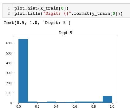
You will notice a thick density of points having value close to zero. These are the black dot points in the image, which obviously is the major portion of the image. The rest of the gray scale points, which are close to white color, represent the digit. You may check out the distribution of pixels for another digit. The code below prints the histogram of a digit at index of 2 in the training dataset.
plot.hist(X_train[2])
plot.title("Digit: {}".format(y_train[2])
The output of running the above code is shown below −
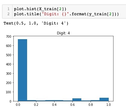
Comparing the above two figures, you will notice that the distribution of the white pixels in two images differ indicating a representation of a different digit - 5 and 4 in the above two pictures.
Next, we will examine the distribution of data in our full training dataset.
Examining Data Distribution
Before we train our machine learning model on our dataset, we should know the distribution of unique digits in our dataset. Our images represent 10 distinct digits ranging from 0 to 9. We would like to know the number of digits 0, 1, etc., in our dataset. We can get this information by using the unique method of Numpy.
Use the following command to print the number of unique values and the number of occurrences of each one
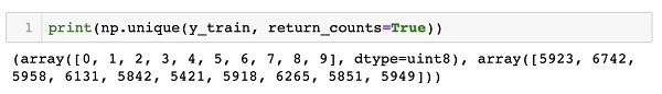
print(np.unique(y_train, return_counts=True))
When you run the above command, you will see the following output −
(array([0, 1, 2, 3, 4, 5, 6, 7, 8, 9], dtype=uint8), array([5923, 6742, 5958, 6131, 5842, 5421, 5918, 6265, 5851, 5949]))
It shows that there are 10 distinct values 0 through 9. There are 5923 occurrences of digit 0, 6742 occurrences of digit 1, and so on. The screenshot of the output is shown here −
As a final step in data preparation, we need to encode our data.
Encoding Data
We have ten categories in our dataset. We will thus encode our output in these ten categories using one-hot encoding. We use to_categorial method of Numpy utilities to perform encoding. After the output data is encoded, each data point would be converted into a single dimensional vector of size 10. For example, digit 5 will now be represented as [0,0,0,0,0,1,0,0,0,0].
Encode the data using the following piece of code −
n_classes = 10
Y_train = np_utils.to_categorical(y_train, n_classes)
You may check out the result of encoding by printing the first 5 elements of the categorized Y_train vector.
Use the following code to print the first 5 vectors −
for i in range(5):
   print (Y_train[i])
You will see the following output −
[0. 0. 0. 0. 0. 1. 0. 0. 0. 0.]
[1. 0. 0. 0. 0. 0. 0. 0. 0. 0.]
[0. 0. 0. 0. 1. 0. 0. 0. 0. 0.]
[0. 1. 0. 0. 0. 0. 0. 0. 0. 0.]
[0. 0. 0. 0. 0. 0. 0. 0. 0. 1.]
The first element represents digit 5, the second represents digit 0, and so on.
Finally, you will have to categorize the test data too, which is done using the following statement −
Y_test = np_utils.to_categorical(y_test, n_classes)
At this stage, your data is fully prepared for feeding into the network.
Next, comes the most important part and that is training our network model.
