Convolution Theorem for Fourier Transform in MATLAB

According to the convolution theorem for Fourier transform, the convolution of two signals in the time domain is equivalent to the multiplication in the frequency domain. Therefore, if two signals are convolved in the time domain, they result the same if their Fourier transforms are multiplied in the frequency domain.

For example, if x(t) and h(t) are two signals in the time domain and their Fourier transforms are X(ω) and H(ω) respectively. Then, their convolution in the time domain is given by,

f(t) = x(t) * h(t)

Here, the symbol ‘*’ represent the convolution of two signals.

And the multiplication of their Fourier transform in the frequency domain is given by,

F(ω) = X(ω).H(ω)

According to the convolution theorem, the functions f(t) and F(ω) are related by the Fourier transform and its inverse as follows.

F(ω) = fft(x(t) * h(t))

And

f(t) = ifft(X(ω).H(ω))

Here, ‘fft’ is a MATLAB function used to perform Fourier transform of the input signals, and ‘ifft’ is another MATLAB function used to perform inverse Fourier transform.

Overall, the convolution theorem for Fourier transform allows us to perform the convolution of input signals in the frequency domain which is simply a multiplication.

Now, let us consider some MATLAB programs to perform the convolution operation in time domain and frequency domain by using the convolution theorem for Fourier transform.

Example

% MATLAB program to demonstrate the use of Convolution Theorem of Fourier Transform
% Define two input signals
x = [2 4 6 8];
y = [0.4 0.4 0.4 0.4];
% Calculate the lengths of the input signals
L1 = length(x);
L2 = length(y);
% Calculate the length of the convolution result
L = L1 + L2 - 1;
% Perform zero-padding of the input signals to the length of the convolution result
a = [x zeros(1, L-L1)];
b = [y zeros(1, L-L2)];
% Perform the Fourier Transform of the padded signals a and b
X = fft(a);
Y = fft(b);
% Perform the convolution in the time domain
CT = conv(x, y);
% Perform the convolution in the frequency domain using the Convolution Theorem
CF = ifft(X .* Y);
% Display the results
disp('Convolution of x and y in the time domain is:');
disp(CT);
disp('Convolution of x and y in the frequency domain using the Convolution Theorem is:');
disp(CF);

Output

Convolution of x and y in the time domain is:
    0.8000    2.4000    4.8000    8.0000    7.2000    5.6000    3.2000

Convolution of x and y in the frequency domain using the Convolution Theorem is:
    0.8000    2.4000    4.8000    8.0000    7.2000    5.6000    3.2000

Explanation

In this MATLAB program, we have defined two input signals stored in variables ‘x’ and ‘y’. Then, we calculate the length of the input signals and the convolution result, and store them in variables ‘L1’, ‘L2’, and ‘L’. Next, we perform zero−padding of signals ‘x’ and ‘y’ to match the length of the convolution result and store the zero−padded signals in variables ‘a’ and ‘b’.

Then, we use the ‘fft’ function to obtain the Fourier transform of zero−padded signals ‘a’ and ‘b’. Next, we perform the convolution of signals ‘x’ and ‘y’ in the time domain by using the ‘conv’ function and store the result in the variable ‘CT’.

After that we perform the multiplication of ‘X’ and ‘Y’ in the frequency domain and calculate the inverse Fourier transform of the product by using the ‘ifft’ function to obtain the convolution result.

Finally, we use the ‘disp’ function to display the results. From the output, we can observe that the results obtained in the time domain, i.e. ‘CT’ and the frequency domain ‘CF’ using the convolution theorem are identical.

Example

% MATLAB program to perform convolution in the spatial domain
% Read the input image
img = imread('https://www.tutorialspoint.com/assets/questions/media/14304-1687425236.jpg');
% Convert the image to grayscale if necessary
if size(img, 3) == 3
    img = rgb2gray(img);
end
% Define averaging filter
filter = ones(10) / 50;
% Perform convolution in the spatial domain
C = conv2(double(img), filter, 'same');
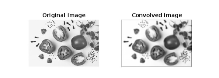
% Display the original and filtered images
subplot(1, 2, 1); imshow(img); title('Original Image');
subplot(1, 2, 2); imshow(C, []); title('Convolved Image');

Output

Explanation

In this MATLAB program, we read the input image by using the ‘imread’ function and store it in a variable ‘img’. Next, we check whether the input image is grayscale or not. If it is not, then we convert it into a grayscale image by using the ‘rgb2gray’ function. Then, we define the averaging filter as a 10 × 10 matrix with all elements set to 1/50, it represents a simple box filter.

After that we perform the convolution of the image in the spatial domain by using the ‘conv2’ function. Here, we also use ‘double()’ function to convert the image to double precision to perform floating calculations.

Finally, we display the original image and the convolved image by using the ‘imshow’ function. Here, ‘[]’ is used to automatically scale the convolved image values.

Example

% MATLAB program to perform convolution in frequency domain
% Read the input image
I = imread('https://www.tutorialspoint.com/assets/questions/media/14304-1687425236.jpg');
% Convert the colored image to grayscale if necessary
if size(I, 3) == 3
    I = rgb2gray(I);
end
% Define averaging filter
filter = ones(10) / 50;
% Calculate the Fourier Transform of the image and the filter
Img_FT = fftshift(fft2(I));
Flt_FT= fftshift(fft2(filter, size(I, 1), size(I, 2)));
% Perform convolution in the frequency domain
C = ifft2(ifftshift(Img_FT .* Flt_FT));
% Display the Fourier Transforms of the image, filter, original image, and convolved image
FT_Image = abs(log(Img_FT));
FT_Filter = abs(log(Flt_FT));
subplot(1, 4, 1), imshow(FT_Image, []); title('FT Image');
subplot(1, 4, 2), imshow(FT_Filter, []); title('FT Filter');
subplot(1, 4, 3), imshow(I, []); title('Original Image');
subplot(1, 4, 4), imshow(C, []); title('Convolved Image');

Output

Explanation

In this MATLAB code, we start by reading the input image by using the ‘imread’ function and store the input image in the ‘I’ variable. Then, we convert the image to a grayscale image if required, for this we use the ‘rgb2gray’ function.

Next, we define the averaging filter ‘filter’ as a 10 × 10 matrix with all elements set to 1/50, it is a simple box filter.

After that we calculate the Fourier transform of the input image and the filter by using the ‘fft2’ function. Here, we also use the ‘fftshift’ function to shift the zero−frequency component to the center for better visualization.

Next, we perform the multiplication of Fourier Transformed Image ‘Img_FT’ and the Fourier Transformed Filter ‘Flt_FT’ in the frequency domain. Also, we calculate the inverse Fourier transform to obtain the convolved image, for this we use the ‘ifft2’ and ‘ifftshift’ functions.

Finally, we display the Fourier transformed image, Fourier transformed filter, original image, and the convolved image by using the ‘imshow’ function. Here, ‘[]’ is used to automatically scale the image values.

Hence, this is all about Convolution Theorem for Fourier Transformer in MATLAB.