- CatBoost - Home
- CatBoost - Overview
- CatBoost - Architecture
- CatBoost - Installation
- CatBoost - Features
- CatBoost - Decision Trees
- CatBoost - Boosting Process
- CatBoost - Core Parameters
- CatBoost - Data Preprocessing
- CatBoost - Handling Categorical Features
- CatBoost - Handling Missing Values
- CatBoost - Classifier
- CatBoost - Model Training
- CatBoost - Metrics for Model Evaluation
- CatBoost - Classification Metrics
- CatBoost - Over-fitting Detection
- CatBoost vs Other Boosting Algorithms
- CatBoost Useful Resources
- CatBoost - Quick Guide
- CatBoost - Useful Resources
- CatBoost - Discussion
CatBoost - Regression
Regression is a machine learning technique that uses previous data to predict numbers such as property prices or the weather for the tomorrow. It shows how several factors, known as variables, influence the number we want to forecast.
For example, when determining the price of a property, relevant considerations include its size, number of bedrooms, and location. To get an accurate prediction regression looks for relationships between these variables and the price.
CatBoost Regression is a specific tool that helps make these predictions. It works well with categorical data, such as different house locations, and is fast and accurate.
Implementation of Regression with CatBoost
So now we are using a dataset to perform a regression work with the help of the CatBoost library. But for using the CatBoost model we will have to first install the CatBoost package model with the help of the below command:
pip install catboost
1. Import required Libraries and Datasets
Now first we will have to import the necessary libraries and the dataset in our code. So here, we will use Python libraries to make it very easy for us to handle the data and perform complex operations using a single line of code. Python libraries like Pandas, numpy, and Matplotlib/Seaborn we are using in our model.
#Import libraries
import pandas as pd
import numpy as np
import seaborn as sb
import matplotlib.pyplot as plt
import lightgbm as lgb

from sklearn.preprocessing import StandardScaler
from sklearn.model_selection import train_test_split

import warnings
warnings.filterwarnings('ignore')
2. Load Dataset and Get Information
Next we are going to load our dataset, here we are using House_Rent_Dataset.csv dataset to predict the House Rent data. So we will load the dataset and print the top 5 rows in the dataset. Check the code below -
# Load dataset here
df = pd.read_csv('/Python/Datasets/House_Rent_Dataset.csv')
print(df.head())
Output
This will produce the following result −
    Posted On  BHK   Rent  Size            Floor    Area Type  \
0  2022-05-18    2  10000  1100  Ground out of 2   Super Area
1  2022-05-13    2  20000   800       1 out of 3   Super Area
2  2022-05-16    2  17000  1000       1 out of 3   Super Area
3  2022-07-04    2  10000   800       1 out of 2   Super Area
4  2022-05-09    2   7500   850       1 out of 2  Carpet Area

              Area Locality     City Furnishing Status  Tenant Preferred  \
0                    Bandel  Kolkata       Unfurnished  Bachelors/Family
1  Phool Bagan, Kankurgachi  Kolkata    Semi-Furnished  Bachelors/Family
2   Salt Lake City Sector 2  Kolkata    Semi-Furnished  Bachelors/Family
3               Dumdum Park  Kolkata       Unfurnished  Bachelors/Family
4             South Dum Dum  Kolkata       Unfurnished         Bachelors

   Bathroom Point of Contact
0         2    Contact Owner
1         1    Contact Owner
2         1    Contact Owner
3         1    Contact Owner
4         1    Contact Owner
Now df.shape will be used to print the dimensions of the dataframe 'df' and df.info() will be used to display the summary about the dataframe 'df'. So it will give details like no. of null entries in each column, data types and also memory usage.
# Print the shape
df.shape

# Show the summary about the DataFrame df
df.info()
Output
This will generate the below result −
(4746, 12)

<class 'pandas.core.frame.DataFrame'>
RangeIndex: 4746 entries, 0 to 4745
Data columns (total 12 columns):
 #   Column             Non-Null Count  Dtype
---  ------             --------------  -----
 0   Posted On          4746 non-null   object
 1   BHK                4746 non-null   int64
 2   Rent               4746 non-null   int64
 3   Size               4746 non-null   int64
 4   Floor              4746 non-null   object
 5   Area Type          4746 non-null   object
 6   Area Locality      4746 non-null   object
 7   City               4746 non-null   object
 8   Furnishing Status  4746 non-null   object
 9   Tenant Preferred   4746 non-null   object
 10  Bathroom           4746 non-null   int64
 11  Point of Contact   4746 non-null   object
dtypes: int64(4), object(8)
memory usage: 445.1+ KB
Now we will generate summary statistics of the DataFrame. So here df.describe() function will be used to calculate and show the basic statistical summary of the numeric columns in the dataframe.
# Generate summary statistics of the DataFrame 'df'
print(df.describe())
Output
This will create the below outcome −
               BHK          Rent         Size     Bathroom
count  4746.000000  4.746000e+03  4746.000000  4746.000000
mean      2.083860  3.499345e+04   967.490729     1.965866
std       0.832256  7.810641e+04   634.202328     0.884532
min       1.000000  1.200000e+03    10.000000     1.000000
25%       2.000000  1.000000e+04   550.000000     1.000000
50%       2.000000  1.600000e+04   850.000000     2.000000
75%       3.000000  3.300000e+04  1200.000000     2.000000
max       6.000000  3.500000e+06  8000.000000    10.000000
EDA (Exploratory Data Analysis)
EDA, which is know as Exploratory Data Analysis, is a method for analyzing data using visual methods. It is used to identify trends and patterns or to validate assumptions through statistical summaries and graphical representations. At the time of the exploratory data analysis (EDA) of the above dataset, we will find the relationships among the independent variables, focusing on how each one affects the others.
# Initialize an empty list
cat_cols = []

# Iterate over DataFrame columns
for col in df.columns:
    if df[col].dtype == 'object' and df[col].nunique() < 10:
        # Add the column to the list
        cat_cols.append(col)
cat_cols += ['BHK', 'Bathroom']
cat_cols
Output
The result of this code is −
['Area Type',
 'City',
 'Furnishing Status',
 'Tenant Preferred',
 'Point of Contact',
 'BHK',
 'Bathroom']
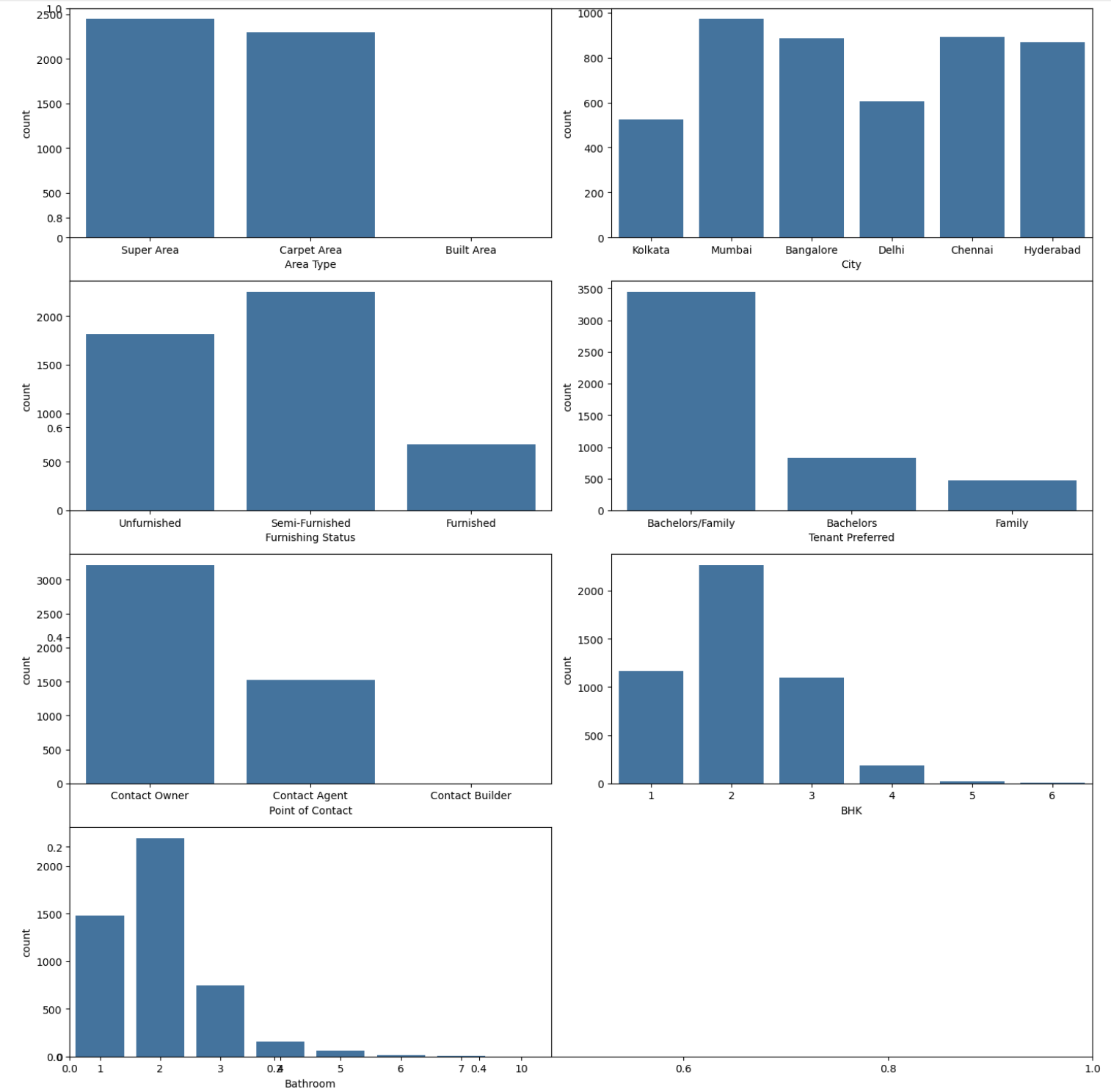
Categorical Count Plots
Next we will observe the distribution of the complete dataset into these categories with the help of a countplot from seaborn. So you need to create subplots to show count plots for categorical columns in 'cat_cols' and subplots will be arranged in a 4x2 grid. And each subplot displays the count distribution for a categorical column.
plt.subplots(figsize=(15, 15))
for i, col in enumerate(cat_cols):
    plt.subplot(4, 2, i+1)
    sb.countplot(data=df, x=col)

# Add proper spacing between subplots
plt.tight_layout()

# Show the subplots
plt.show()
Output
In the below output image you can see each plot shows the distribution of counts for a specific categorical column. The "plt. tight_layout" function makes sure proper spacing between subplots and the 'plt_show' shows the grid of count plots.
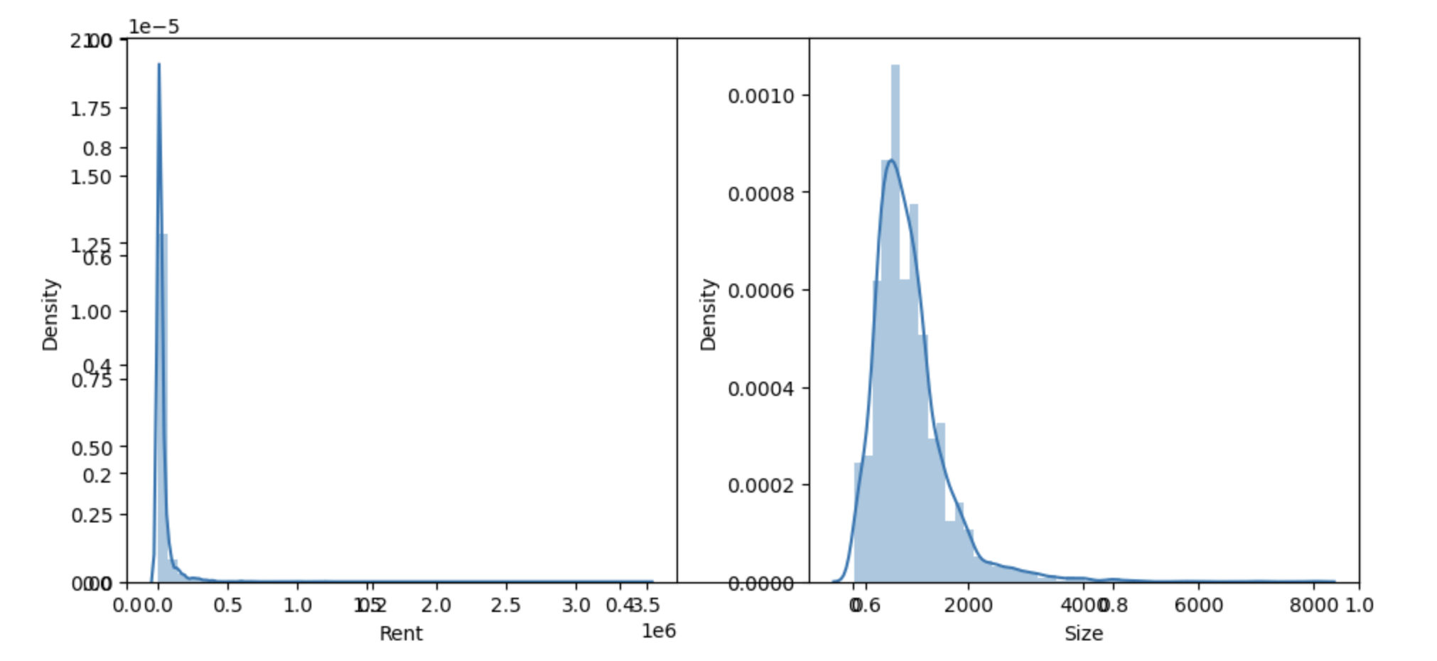
Numeric Distribution Plots
To understand numerical data and its distribution the density plots are used as one of the most effective tools. So create subplots to present distribution plots for numeric columns in 'num_cols'.
num_cols = ['Rent', 'Size']
plt.subplots(figsize=(10, 5))
for i, col in enumerate(num_cols):
    plt.subplot(1, 2, i+1)
    sb.distplot(df[col])
plt.tight_layout()
plt.show()
Output
In the below output images, we can see that both the rent and the size columns are not normally distributed, and it considered best practice to have the target and features columns frequently distributed for better results when using regressions in machine learning. One well-known way of doing this is logarithmic transformation.
Now we will remove the unnecessary columns from the dataset. We can draw the following observations from this dataset −
Carpeted houses get more rentals than others.
Rents in major cities like Mumbai and Delhi are too high.
Furnished apartments cost more than unfurnished or semi-furnished apartments.
Renting a property via an agent looks to have the highest value, which is owing to the commission needed to get the property.
Charges for family members are higher than for bachelors.
Rents often rise as the number of bathrooms and BHK sizes in the area increases.
Most of the observations we made above match what we see in real life.
df.drop(['Posted On', 'Floor', 'Area Locality'],
        inplace=True, axis=1)

# Calculate and show the mean rent for every category
for i, col in enumerate(cat_cols):
    print(df[[col, 'Rent']].groupby(col).mean())
    print()
Output
The result of this PHP code is −
                     Rent
Area Type
Built Area   10500.000000
Carpet Area  52385.897302
Super Area   18673.396566

                   Rent
City
Bangalore  24966.365688
Chennai    21614.092031
Delhi      29461.983471
Hyderabad  20555.048387
Kolkata    11645.173664
Mumbai     85321.204733

                           Rent
Furnishing Status
Furnished          56110.305882
Semi-Furnished     38718.810751
Unfurnished        22461.635813

                          Rent
Tenant Preferred
Bachelors         42143.793976
Bachelors/Family  31210.792683
Family            50020.341102

                          Rent
Point of Contact
Contact Agent     73481.158927
Contact Builder    5500.000000
Contact Owner     16704.206468

              Rent
BHK
1     14139.223650
2     22113.864018
3     55863.062842
4    168864.555556
5    297500.000000
6     73125.000000

                   Rent
Bathroom
1          11862.162144
2          25043.538193
3          63176.698264
4         167846.153846
5         252350.000000
6         177500.000000
7          81666.666667
10        200000.000000
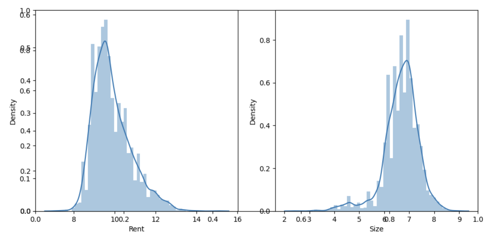
Data Preprocessing
Data preparation is important in any ML development lifecycle because we know that the real-world dataset is disorganized, and before we can use it, we must convert it to structural form and use it in a way that allows us to extract value from it.
With the current data, we will first apply the logarithmic transformation to the rent and size columns, which are left skewed rather than normally distributed.
# Log-transform
num_cols = ['Rent', 'Size']
df[num_cols] = np.log1p(df[num_cols])

# Create subplots
plt.subplots(figsize=(10, 5))
for i, col in enumerate(num_cols):
    plt.subplot(1, 2, i+1)
    sb.distplot(df[col])

# Add proper space
plt.tight_layout()

# Show the subplots
plt.show()
Output
To reduce data skewness, this code uses np.log1p to the "Rent" and "Size" columns. The distribution of values in each column can be seen on distribution plots for the log-transformed numerical columns. Finally the distribution plots subplots are presented using 'plt.show()'.
One-Hot Encoding Categorical Columns
One hot encoding is seen as the ideal strategy for converting categorical columns to numerical ones because, unlike the ordinal encoding method, no category is given higher priority in this process.
cat_cols = ['Area Type', 'City', 'Furnishing Status',
            'Point of Contact', 'Tenant Preferred']

for col in cat_cols:
    temp = pd.get_dummies(df[col]).astype('int')
    df = pd.concat([df, temp], axis=1)

df.drop(cat_cols, axis=1, inplace=True)
print(df.head())
Output
This will lead to the following outcome −
   BHK      Rent      Size  Bathroom  Built Area  Carpet Area  Super Area  \
0    2  9.210440  7.003974         2           0            0           1
1    2  9.903538  6.685861         1           0            0           1
2    2  9.741027  6.908755         1           0            0           1
3    2  9.210440  6.685861         1           0            0           1
4    2  8.922792  6.746412         1           0            1           0
   Bangalore  Chennai  Delhi  ...  Mumbai  Furnished  Semi-Furnished  \
0          0        0      0  ...       0          0               0
1          0        0      0  ...       0          0               1
2          0        0      0  ...       0          0               1
3          0        0      0  ...       0          0               0
4          0        0      0  ...       0          0               0
   Unfurnished  Contact Agent  Contact Builder  Contact Owner  Bachelors  \
0            1              0                0              1          0
1            0              0                0              1          0
2            0              0                0              1          0
3            1              0                0              1          0
4            1              0                0              1          1
   Bachelors/Family  Family
0                 1       0
1                 1       0
2                 1       0
3                 1       0
4                 0       0
[5 rows x 22 columns]
Splitting Data
We will now divide the entire dataset into training and validation parts using an 85:15 ratio.
# Split the Dataset
# Features (independent variables)
features = df.drop('Rent', axis=1)
# Target variable
target = df['Rent']

# Split the data into training and testing datasets
X_train, X_val, Y_train, Y_val = train_test_split(
    features, target, random_state=2023, test_size=0.15)

# Show the shapes of the training and testing datasets
X_train.shape, X_val.shape
Output
This will create the below outcome −
((4034, 21), (712, 21))
Model Development
Now that we have all of the data ready, it is being preprocessed and divided into training and testing datasets. Now we will import the catboostregressor from the catboost module and train it on our data.
'CatBosstRegressor' is a Python class offered by the catboost package for building regression models. It is specifically developed for regression jobs, which need the code to predict a continuous numeric target variable based on input data.
The code 'CatBoostRegressor(loss function='RMSE')' initializes the Catboost regression model using the Root Mean Squared Error (RMSE) as the loss function. The model's goal is to minimize errors during training.
# CatBoost Regression Model
from catboost import CatBoostRegressor

# Initialize the CatBoostRegressor
model = CatBoostRegressor(loss_function='RMSE')

# Fit the model
model.fit(X_train, Y_train, verbose=100)
Output
As we can see in the below result, the training has been completed for approximately 1000 epochs, and we are able to use the training and testing data to evaluate the model's performance.
Learning rate set to 0.051037
0:	learn: 0.8976462	total: 59.3ms	remaining: 59.3s
100:	learn: 0.3741647	total: 205ms	remaining: 1.83s
200:	learn: 0.3571139	total: 315ms	remaining: 1.25s
300:	learn: 0.3455686	total: 424ms	remaining: 984ms
400:	learn: 0.3369937	total: 541ms	remaining: 808ms
500:	learn: 0.3305270	total: 653ms	remaining: 650ms
600:	learn: 0.3252100	total: 768ms	remaining: 510ms
700:	learn: 0.3200064	total: 886ms	remaining: 378ms
800:	learn: 0.3153692	total: 1.01s	remaining: 251ms
900:	learn: 0.3116973	total: 1.13s	remaining: 124ms
999:	learn: 0.3082544	total: 1.24s	remaining: 0us
<catboost.core.CatBoostRegressor at 0x13a8cd700>
Prediction
Here, we can see that before passing the data to the model we have converted the categorical features to numerical or hot encoded ones. However when using the catboost model, we can choose not to do this step directly.
# Import the mean squared error (MSE) function
from sklearn.metrics import mean_squared_error as mse

# Generate predictions on the training and testing datasets
y_train = model.predict(X_train)
y_val = model.predict(X_val)

# Calculate and print the RMSE
print("Training the RMSE: ", np.sqrt(mse(Y_train, y_train)))
print("Validation the RMSE: ", np.sqrt(mse(Y_val, y_val)))
Output
This will produce the following result −
Training the RMSE:  0.30825444436592375
Validation the RMSE:  0.39986315317196297
