CatBoost - Model Training

---

---

CatBoost is a high-performance gradient-boosting method created for machine learning applications, specifically ones that need structured input. Gradient boosting forms the foundation of its main process. Usually, CatBoost begins by making assumptions about the mean of the target variable.

The next stage is to progressively build the ensemble of decision trees, with each tree seeking to remove the residuals or errors from the previous one. CatBoost is different in the way it handles categorical features. CatBoost uses a technique called "ordered boosting" to evaluate category input directly, improving model performance and simplifying training.

Additionally, regularization methods are used to prevent overfitting. CatBoost combines calculated values from every tree to create predictions, generating highly precise and stable models. Also, it provides feature relevance scores to help with understanding of feature and model selections. CatBoost is a valuable tool for a number of machine-learning problems like regression and classification.

So let us see how we can train the CatBoost model in this chapter −

Implementation Using CatBoost

To use CatBoost you need to install it in your system. To install you can use 'pip install catboost'. Type this command on your terminal and the package will be installed automatically.

Import required Libraries and Dataset

So you have to import the required libraries to build your model. Also we are using placement dataset to build our model in this chapter. So will load the data into the pandas dataframe and display it using the pd.read_csv() function. Let us see how we can do this −

import pandas as pd
import numpy as np
import seaborn as sb
import matplotlib.pyplot as plt

from sklearn.preprocessing import StandardScaler
from sklearn.model_selection import train_test_split
from catboost import CatBoostClassifier
from sklearn.metrics import roc_auc_score as ras

import warnings
warnings.filterwarnings('ignore')

# Load you dataset here
df = pd.read_csv('placementdata.csv')
print(df.head())

Output

This code will produce the following outcome −

   StudentID  CGPA  Internships  Projects  Workshops/Certifications  \
0          1   7.5            1         1                         1   
1          2   8.9            0         3                         2   
2          3   7.3            1         2                         2   
3          4   7.5            1         1                         2   
4          5   8.3            1         2                         2   

   AptitudeTestScore  SoftSkillsRating ExtracurricularActivities  \
0                 65               4.4                        No   
1                 90               4.0                       Yes   
2                 82               4.8                       Yes   
3                 85               4.4                       Yes   
4                 86               4.5                       Yes   

  PlacementTraining  SSC_Marks  HSC_Marks PlacementStatus  
0                No         61         79       NotPlaced  
1               Yes         78         82          Placed  
2                No         79         80       NotPlaced  
3               Yes         81         80          Placed  
4               Yes         74         88          Placed  

If we take the time to look at the data above, we can see that this dataset contains information about the students' academic, training, and placement status.

Shape And Info of the Dataset

Let us now find out the structure and information of the dataset in order to calculate the total number of data entries that have been given. The content of each column, the data types that are present in it, and the amount of null values that are present in each column can all be seen by using the df.info() method.

# Shape of the dataset
df.shape

# Information of the dataset
df.info()

Output

This will result in the following outcome −

(10000, 12)

<class 'pandas.core.frame.DataFrame'>
RangeIndex: 10000 entries, 0 to 9999
Data columns (total 12 columns):
 #   Column                     Non-Null Count  Dtype  
---  ------                     --------------  -----  
 0   StudentID                  10000 non-null  int64  
 1   CGPA                       10000 non-null  float64
 2   Internships                10000 non-null  int64  
 3   Projects                   10000 non-null  int64  
 4   Workshops/Certifications   10000 non-null  int64  
 5   AptitudeTestScore          10000 non-null  int64  
 6   SoftSkillsRating           10000 non-null  float64
 7   ExtracurricularActivities  10000 non-null  object 
 8   PlacementTraining          10000 non-null  object 
 9   SSC_Marks                  10000 non-null  int64  
 10  HSC_Marks                  10000 non-null  int64  
 11  PlacementStatus            10000 non-null  object 
dtypes: float64(2), int64(7), object(3)
memory usage: 937.6+ KB

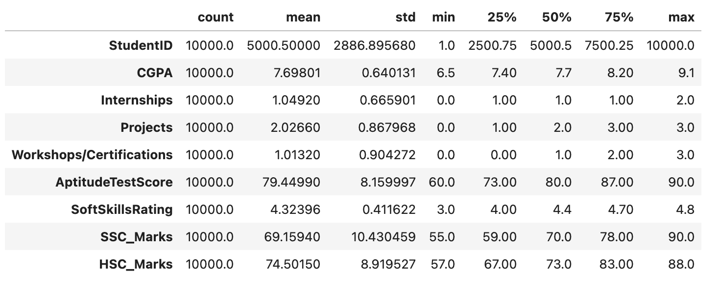
The DataFrame df is statistically represented by the df.describe() function. Key statistics, like count, mean, standard deviation, minimum, and maximum values, are given for each numerical column to give an initial understanding of the data distribution and primary patterns.

df.describe().T

Output

This code will produce the following outcome −

Exploratory Data Analysis(EDA)

EDA is a data analysis technique that uses visualizations. It is used to identify trends and patterns as well as to confirm conclusions with the use of statistical reports and graphical representations. While performing the EDA on this dataset, we will try to find out the relationship that is, how one effects the other between the independent features.

Let us start by taking a quick look at the null values in each column of the data frame.

df.isnull().sum()

Output

This code will generate the below outcome −

StudentID                    0
CGPA                         0
Internships                  0
Projects                     0
Workshops/Certifications     0
AptitudeTestScore            0
SoftSkillsRating             0
ExtracurricularActivities    0
PlacementTraining            0
SSC_Marks                    0
HSC_Marks                    0
PlacementStatus              0
dtype: int64

Since there are no null values in the dataset, we can continue with the data exploration.

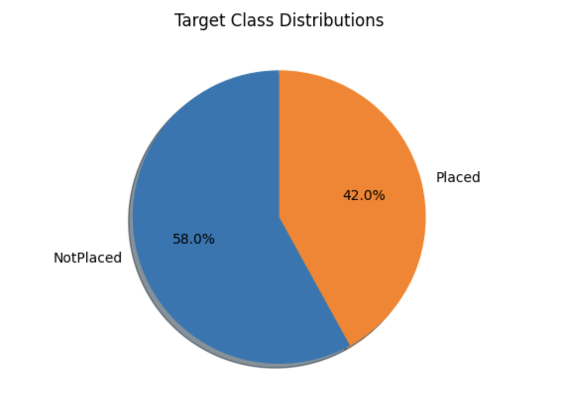
Target Class Distributions

temporary = df['PlacementStatus'].value_counts()

plt.pie(temporary.values, labels=temporary.index.values,
	shadow=True, startangle=90, autopct='%1.1f%%')
plt.title("Target Class Distributions")

plt.show()

Output

The pie chart below displays the approximately balanced class distribution of the dataset. While this may not be perfect, it is still acceptable. The dataset includes both category and number columns, as we can see. Let us divide the dataset into two lists before we look at these attributes.

Divide the Columns

Now we will be dividing the columns of a DataFrame (df) in two main categories- categorical columns and numerical columns.

categorical_columns, numerical_columns = list(), list()

for col in df.columns:
   if df[col].dtype == 'object' or df[col].nunique() < 10:
      categorical_columns.append(col)
   else:
      numerical_columns.append(col)

print('Categorical Columns:', categorical_columns)
print('Numerical Columns:', numerical_columns)

Output

This code will produce the following outcome −

Categorical Columns: ['Internships', 'Projects', 'Workshops/Certifications', 'ExtracurricularActivities', 'PlacementTraining', 'PlacementStatus']
Numerical Columns: ['StudentID', 'CGPA', 'AptitudeTestScore', 'SoftSkillsRating', 'SSC_Marks', 'HSC_Marks']

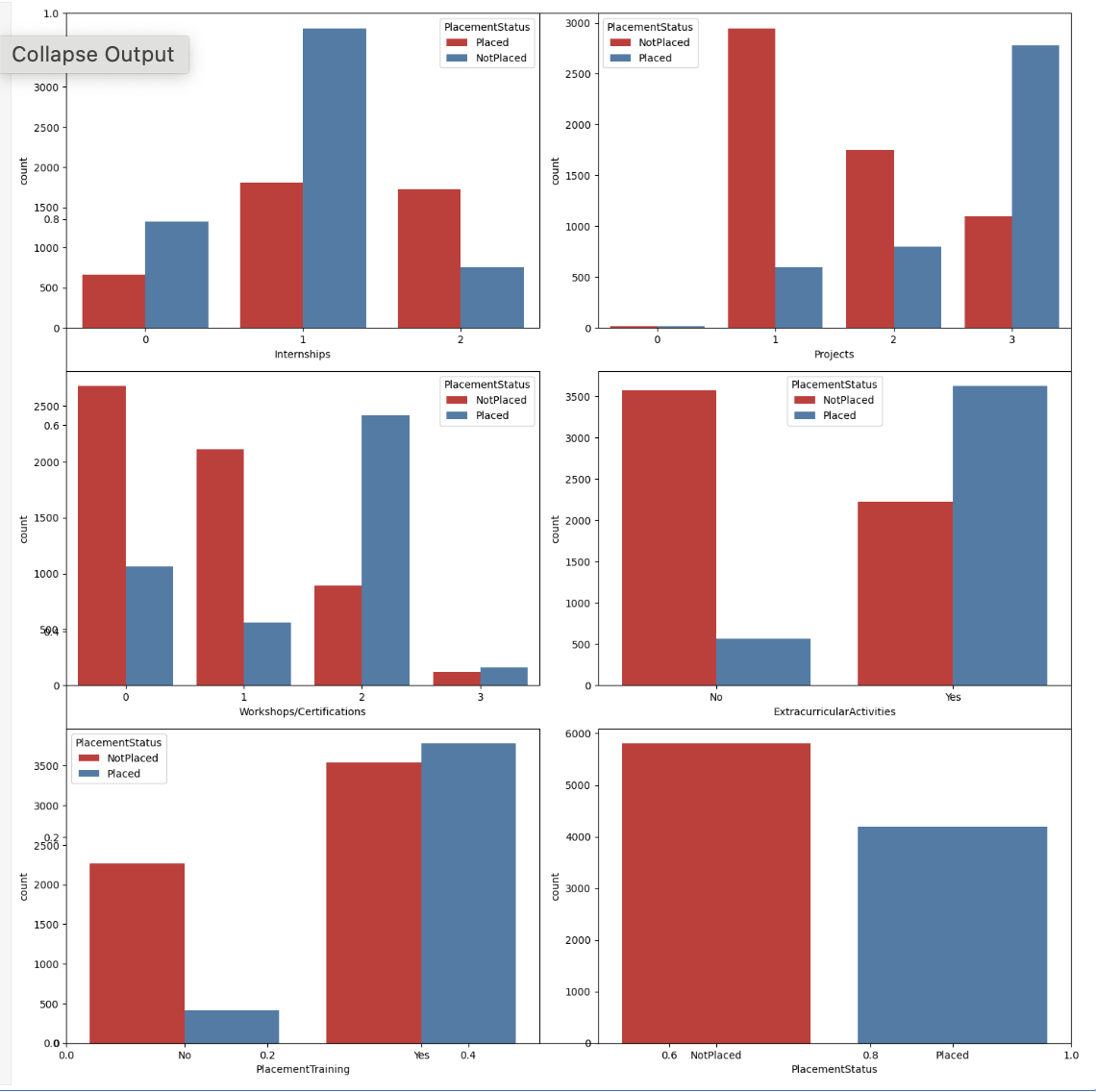
Countplot for Categorical Columns

Now we will create countplot for the Categorical Columns with the help of the hue of placement status.

plt.subplots(figsize=(15, 15))

for i, col in enumerate(categorical_columns):
   plt.subplot(3, 2, i+1)
   sb.countplot(data=df, x=col, hue='PlacementStatus', palette='Set1') 
plt.tight_layout()
plt.show()

Output

The charts provided shown below show multiple patterns that support the idea that focusing on your skill development will surely help with your placement. While it is true that some students have completed training courses and projects and are still not placed, this is a relatively small number in comparison to those who have done nothing.

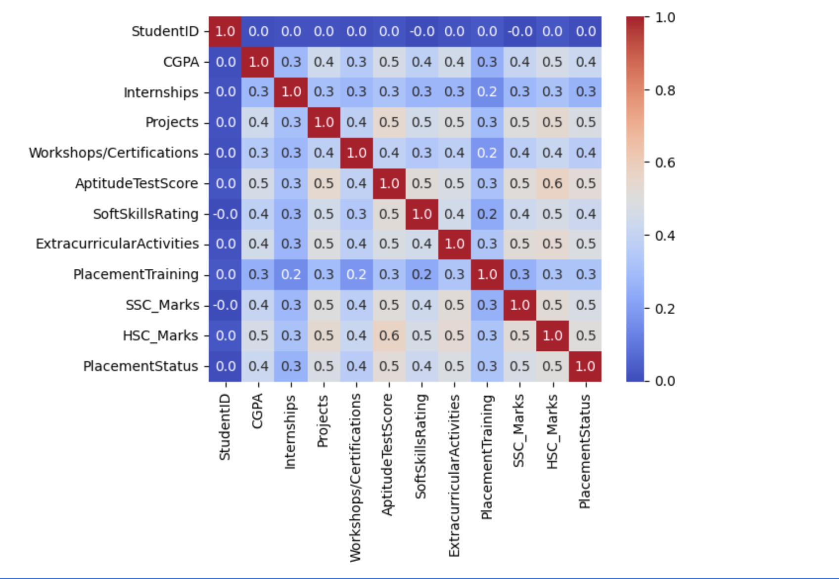
Label Encoding of Categorical Columns

After the encoding of the dataset's categorical features, we will create a heatmap that will help in identifying the highly correlated characteristics inside the feature space with the target columns.

for col in ['ExtracurricularActivities', 'PlacementTraining']:
   df[col] = df[col].map({'No':0,'Yes':1})
     
df['PlacementStatus']=df['PlacementStatus'].map({'NotPlaced':0, 'Placed':1})

Confusion Matrix

Now we will create the confusion matrix for the above dataset.

sb.heatmap(df.corr(), fmt='.1f', cbar=True, annot=True, cmap='coolwarm')  
plt.show()

Output

The below outcome shows that there is no data leakage because the dataset does not contain any highly connected or correlated features.

Train and Validations Data Split

Let us divide the dataset in an 85:15 ratio in order to figure out the model's performance during training. This allows us evaluate the model's performance using the validation split's unseen dataset.

features = df.drop(['StudentID', 'PlacementStatus'], axis=1)
target = df['PlacementStatus']
 
X_train, X_val, Y_train, Y_val = train_test_split(
   features, 
   target,
   random_state=2023,
   test_size=0.15)
 
X_train.shape, X_val.shape

Output

This will bring about the following outcome −

((8500, 10), (1500, 10))

Feature scaling

This code fits the StandardScaler to the training data in order to compute the mean and standard deviation, providing consistent scaling between the two datasets. After that it uses these computed values to convert the training and validation data.

scaler = StandardScaler()
scaler.fit(X_train)
X_train = scaler.transform(X_train)
X_val = scaler.transform(X_val)

Build and Train the Model

We can now start training the model with the available training data. Since there are only two possible values in the target columns, Y_train and Y_val, binary classification is being performed in this case. Separate specifications are not needed whether the model is being trained for a binary or multi-class classification task.

ourmodel = CatBoostClassifier(verbose=100,
	iterations=1000,
	loss_function='Logloss',
	early_stopping_rounds=50,
	custom_metric=['AUC'])

ourmodel.fit(X_train, Y_train,
	eval_set=(X_val, Y_val))

y_train = ourmodel.predict(X_train)
y_val = ourmodel.predict(X_val)

Output

This will lead to the following outcome −

Learning rate set to 0.053762
0:	learn: 0.6621705	test: 0.6623146	best: 0.6623146 (0)	total: 64.3ms	remaining: 1m 4s
100:	learn: 0.3975289	test: 0.4332971	best: 0.4332174 (92)	total: 230ms	remaining: 2.05s
Stopped by overfitting detector  (50 iterations wait)

bestTest = 0.4330066724
bestIteration = 125

Shrink model to first 126 iterations.

Evaluate Model's Performance

Now let us use the ROC AUC measure to evaluate the model's performance on the training and validation data sets.

print("Training ROC AUC: ", ras(Y_train, y_train))
print("Validation ROC AUC: ", ras(Y_val, y_val))

Output

This will bring about the following outcome −

Training ROC AUC:  0.8175316989019953
Validation ROC AUC:  0.7859439713002392