
 Data Structure
 Networking
 RDBMS
RDBMS Operating System
 Java
Java MS Excel
 iOS
iOS HTML
HTML CSS
CSS Android
 Python
 C Programming
 C++
C++ C#
C# MongoDB
 MySQL
MySQL Javascript
 PHP
PHP
- Selected Reading
- UPSC IAS Exams Notes
- Developer's Best Practices
- Questions and Answers
- Effective Resume Writing
- HR Interview Questions
- Computer Glossary
- Who is Who
What is Mesh Current Analysis?
In this method, Kirchhoff’s voltage law is applied to a network to write mesh equations in terms of mesh currents. The branch currents are then found by taking the algebraic sum of the mesh currents which are common to that branch.
Kirchhoff’s Voltage Law
The Kirchhoff’s voltage law (KVL) states that, the algebraic sum of all the emfs and voltage drops is equal to zero in a mesh i.e.
$$\mathrm{\sum\:emfs\:+\:\sum\:Voltage\:Drops = 0}$$
Mesh − A mesh is a most elementary form of a loop, which cannot be further divided into other loops i.e. a mesh does not have any inner loop.
Explanation
Each mesh is assigned a separate mesh current. For convenience, all mesh currents are assumed to flow in one direction (clockwise or anticlockwise). The same results will be obtained if the mesh currents are given arbitrary directions.
If two mesh currents are flowing through a circuit element, the actual current in the element is the algebraic sum of the two currents.
KVL is applied to write equations for each mesh in terms of mesh currents. While writing the mesh equations, the rise in potential is assigned positive sign and fall in potential negative sign.
If the value of any mesh current comes out to be negative in the solution, it means that, the true direction of that mesh current is opposite to the assumed direction.
Applying KVL in the circuit shown below to write the mesh equations, as
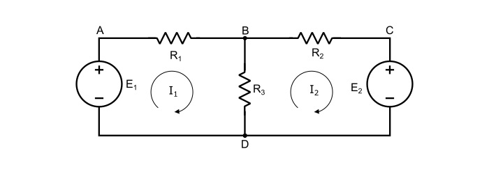
Applying KVL in mesh ABDA,
$$\mathrm{\mathit{E}_{1}-\mathit{I}_{1}\mathit{R}_{1}-(\mathit{I}_{1}-\mathit{I}_{2})\mathit{R}_{3}=0}$$
$$\mathrm{\Rightarrow\:\mathit{E}_{1}=\mathit{I}_{1}\mathit{R}_{1}-(\mathit{I}_{1}-\mathit{I}_{2})\mathit{R}_{3}}$$
$$\mathrm{\Rightarrow\:\mathit{E}_{1}=\mathit{I}_{1}(\mathit{R}_{1}\:+\:\mathit{R}_{3})-\mathit{I}_{2}\mathit{R}_{3}}\:\:\:… (1)$$
Applying KVL in mesh BCDB,
$$\mathrm{-\mathit{I}_{2}\mathit{R}_{2}-\mathit{E}_{2}(\mathit{I}_{2}-\mathit{I}_{1})\mathit{R}_{3}=0}$$
$$\mathrm{\Rightarrow\:\mathit{E}_{2}=\mathit{I}_{1}\mathit{R}_{3}-\mathit{I}_{2}(\mathit{R}_{2}\:+\:\mathit{R}_{3})}\:\:\:… (2)$$
By solving equations (1) and (2) simultaneously, the mesh currents I1 and I2 can be obtained. Once the mesh currents are obtained, the currents through the branches of the circuit can be readily found out.
Note – The mesh currents are imaginary quantities and cannot be measured. Whereas, the branch currents are the real currents because they actually flow in the branches and can be measured.
Numerical Example
Calculate the current in each branch of the circuit shown below.
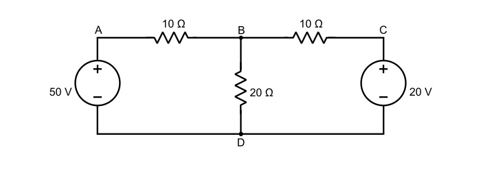
Solution
Assign mesh currents I1 and I2 to meshes ABDA and BCDB respectively as shown in the circuit below.
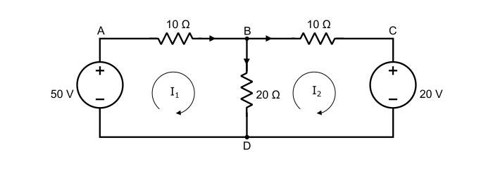
Applying KVL to the mesh ABDA,
$$\mathrm{50-10\mathit{I}_{1}-20(\mathit{I}_{1}-\mathit{I}_{2})=0}$$
$$\mathrm{\Rightarrow\:50=30\mathit{I}_{1}-20\mathit{I}_{2}}$$
$$\mathrm{3\mathit{I}_{1}-2\mathit{I}_{2}=5\:\:\:… (3)}$$
Applying KVL to the mesh BCDB,
$$\mathrm{-10\mathit{I}_{2}-20-20(\mathit{I}_{2}-\mathit{I}_{1})=0}$$
$$\mathrm{\Rightarrow\:-30\mathit{I}_{2}+20\mathit{I}_{1}=20}$$
$$\mathrm{2\mathit{I}_{1}-3\mathit{I}_{2}=2\:\:\:… (4)}$$
Solving equation (3) and (4) simultaneously, the mesh currents I1 and I2 are,
$$\mathrm{\mathit{I}_{1}=2.2\:A\:and\:\mathit{I}_{2}=0.8\:A}$$
Hence, the branch currents will be,
$$\mathrm{Current\:in\:the\:branch\:DAB=\mathit{I}_{1}=2.2\:A\:\:\:(flows\:from\:A\:to\:B)}$$
$$\mathrm{Current\:in\:the\:branch\:BCD=\mathit{I}_{2}=0.8\:A\:\:\:(flows\:from\:B\:to\:C)}$$
$$\mathrm{Current\:in\:the\:branch\:BD=(\mathit{I}_{1}-I_{2})=2.2 − 0.8 = 1.4\:A\:\:\:(flows\:from\:B\:to\:D)}$$

824 Views
