What is Computational Model?

It is widely observed that certain computer architecture classes and programming language classes correspond to one another. For example von Neumann architectures and imperative languages, or reduction architectures and functional languages. The corresponding architecture and language classes must have a common foundation or paradigm called a computational model.

The computational model comprises the set of following three abstractions are as shown in the figure −

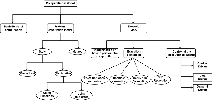
The first abstraction identifies the basic items of computation. This is a specification of the items the computation refers to any kind of computations that can be performed on them.

For instance, in the Von Neumann computational model, the basic items of computations are data. This data will typically be represented by named entities to be able to distinguish between several different data items in the course of a computation. These named entities are commonly called variables in programming languages and are implemented by memory or register addresses in architectures.

The problem description model refers to both the style and method of problem description as shown in the figure.

The problem description style specifies how problems in a particular computational model are described. The style is either procedural or declarative as shown in the figure.

In a procedural style, the algorithm for solving the problem is stated. A particular solution is then declared in the form of an algorithm.

If a declarative style is used, all the facts and relationships relevant to the given problem have to be stated. There are two methods for expressing this relationship and facts. The first uses functions, as in the applicative model of computation, while the second states the relationships and facts in the form of predicates, as in the predicate-logic-based computation model.

The other component of the problem description model is the problem description method. It is interpreted differently for the procedural and declarative styles. When using the procedural style the problem description model states how a solution to the given problem has to be described.

While using a declarative style, it specifies how the problem itself has to be described. For instance, in the Von Neumann computational model, a problem solution is described as a sequence of instructions expressing an appropriate algorithm.

Execution Model − The last element of the computational model is the execution model. The first component declares the interpretation of the computation, which is strongly related to the problem description method. The choice of problem description method and the interpretation of the computation mutually determine and presume each other.

The next component of the execution model specifies the execution semantics. This can be interpreted as a rule that prescribes how a single execution step is to be performed.

There are different types of execution semantics applied by the basic computational model are shown in the figure. State transition semantics is used in Turing, von Neumann, and object-based models, data flow semantics in the corresponding dataflow model, reduction semantics in the applicative model, and the SLD-resolution in the predicate logic-based computational model.

The last component of the model specifies the control of the execution sequence. In the basic models, execution is either control driver or data-driven or demand-driven.

Control-Driven Execution − It is assumed that there exists a program consisting of a sequence of instructions. The execution sequence is then implicitly given by the order of the instructions.

Data-Driven Execution − It is characterized by the rule that an operation is activated as soon as all the needed input data is available. This model of the sequence is also called eager evaluation.

Demand-Driven Execution − In demand-driven execution, the operation will be activated only when their execution is needed to achieve the final result. This mode of execution control is also called lazy evaluation because the delayed until needed philosophy is applied.