- Theano - Home
- Theano - Introduction
- Theano - Installation
- Theano - A Trivial Theano Expression
- Theano - Expression for Matrix Multiplication
- Theano - Computational Graph
- Theano - Data Types
- Theano - Variables
- Theano - Shared Variables
- Theano - Functions
- Theano - Trivial Training Example
- Theano - Conclusion
- Theano Useful Resources
- Theano - Quick Guide
- Theano - Useful Resources
- Theano - Discussion
Theano - Quick Guide
Theano - Introduction
Have you developed Machine Learning models in Python? Then, obviously you know the intricacies in developing these models. The development is typically a slow process taking hours and days of computational power.
The Machine Learning model development requires lot of mathematical computations. These generally require arithmetic computations especially large matrices of multiple dimensions. These days we use Neural Networks rather than the traditional statistical techniques for developing Machine Learning applications. The Neural Networks need to be trained over a huge amount of data. The training is done in batches of data of reasonable size. Thus, the learning process is iterative. Thus, if the computations are not done efficiently, training the network can take several hours or even days. Thus, the optimization of the executable code is highly desired. And that is what exactly Theano provides.
Theano is a Python library that lets you define mathematical expressions used in Machine Learning, optimize these expressions and evaluate those very efficiently by decisively using GPUs in critical areas. It can rival typical full C-implementations in most of the cases.
Theano was written at the LISA lab with the intention of providing rapid development of efficient machine learning algorithms. It is released under a BSD license.
In this tutorial, you will learn to use Theano library.
Theano - Installation
Theano can be installed on Windows, MacOS, and Linux. The installation in all the cases is trivial. Before you install Theano, you must install its dependencies. The following is the list of dependencies −
- Python
- NumPy − Required
- SciPy − Required only for Sparse Matrix and special functions
- BLAS − Provides standard building blocks for performing basic vector and matrix operations
The optional packages that you may choose to install depending on your needs are −
- nose: To run Theanos test-suite
- Sphinx − For building documentation
- Graphiz and pydot − To handle graphics and images
- NVIDIA CUDA drivers − Required for GPU code generation/execution
- libgpuarray − Required for GPU/CPU code generation on CUDA and OpenCL devices
We shall discuss the steps to install Theano in MacOS.
MacOS Installation
To install Theano and its dependencies, you use pip from the command line as follows. These are the minimal dependencies that we are going to need in this tutorial.
$ pip install Theano
$ pip install numpy
$ pip install scipy
$ pip install pydot
You also need to install OSx command line developer tool using the following command −
$ xcode-select --install
You will see the following screen. Click on the Install button to install the tool.

On successful installation, you will see the success message on the console.
Testing the Installation
After the installation completes successfully, open a new notebook in the Anaconda Jupyter. In the code cell, enter the following Python script −
Example
import theano
from theano import tensor
a = tensor.dscalar()
b = tensor.dscalar()
c = a + b
f = theano.function([a,b], c)
d = f(1.5, 2.5)
print (d)
Output
Execute the script and you should see the following output −
4.0
The screenshot of the execution is shown below for your quick reference −
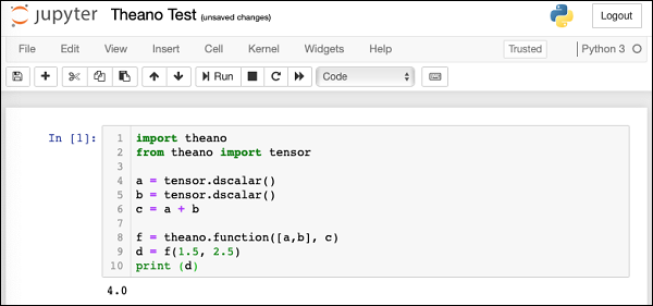
If you get the above output, your Theano installation is successful. If not, follow the debug instructions on Theano download page to fix the issues.
What is Theano?
Now that you have successfully installed Theano, let us first try to understand what is Theano? Theano is a Python library. It lets you define, optimize, and evaluate mathematical expressions, especially the ones which are used in Machine Learning Model development. Theano itself does not contain any pre-defined ML models; it just facilitates its development. It is especially useful while dealing with multi-dimensional arrays. It seamlessly integrates with NumPy, which is a fundamental and widely used package for scientific computations in Python.
Theano facilitates defining mathematical expressions used in ML development. Such expressions generally involve Matrix Arithmetic, Differentiation, Gradient Computation, and so on.
Theano first builds the entire Computational Graph for your model. It then compiles it into highly efficient code by applying several optimization techniques on the graph. The compiled code is injected into Theano runtime by a special operation called function available in Theano. We execute this function repetitively to train a neural network. The training time is substantially reduced as compared to using pure Python coding or even a full C implementation.
We shall now understand the process of Theano development. Let us begin with how to define a mathematical expression in Theano.
Theano - A Trivial Theano Expression
Let us begin our journey of Theano by defining and evaluating a trivial expression in Theano. Consider the following trivial expression that adds two scalars −
c = a + b
Where a, b are variables and c is the expression output. In Theano, defining and evaluating even this trivial expression is tricky.
Let us understand the steps to evaluate the above expression.
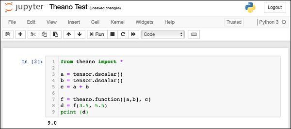
Importing Theano
First, we need to import Theano library in our program, which we do using the following statement −
from theano import *
Rather than importing the individual packages, we have used * in the above statement to include all packages from the Theano library.
Declaring Variables
Next, we will declare a variable called a using the following statement −
a = tensor.dscalar()
The dscalar method declares a decimal scalar variable. The execution of the above statement creates a variable called a in your program code. Likewise, we will create variable b using the following statement −
b = tensor.dscalar()
Defining Expression
Next, we will define our expression that operates on these two variables a and b.
c = a + b
In Theano, the execution of the above statement does not perform the scalar addition of the two variables a and b.
Defining Theano Function
To evaluate the above expression, we need to define a function in Theano as follows −
f = theano.function([a,b], c)
The function function takes two arguments, the first argument is an input to the function and the second one is its output. The above declaration states that the first argument is of type array consisting of two elements a and b. The output is a scalar unit called c. This function will be referenced with the variable name f in our further code.
Invoking Theano Function
The call to the function f is made using the following statement −
d = f(3.5, 5.5)
The input to the function is an array consisting of two scalars: 3.5 and 5.5. The output of execution is assigned to the scalar variable d. To print the contents of d, we will use the print statement −
print (d)
The execution would cause the value of d to be printed on the console, which is 9.0 in this case.
Full Program Listing
The complete program listing is given here for your quick reference −
from theano import *
a = tensor.dscalar()
b = tensor.dscalar()
c = a + b
f = theano.function([a,b], c)
d = f(3.5, 5.5)
print (d)
Execute the above code and you will see the output as 9.0. The screen shot is shown here −
Now, let us discuss a slightly more complex example that computes the multiplication of two matrices.
Theano - Expression for Matrix Multiplication
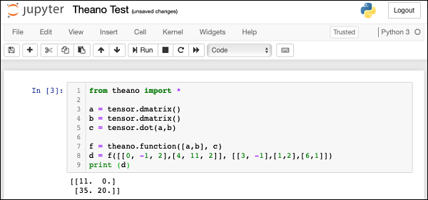
We will compute a dot product of two matrices. The first matrix is of dimension 2 x 3 and the second one is of dimension 3 x 2. The matrices that we used as input and their product are expressed here −
$$\begin{bmatrix}0 & -1 & 2\\4 & 11 & 2\end{bmatrix} \:\begin{bmatrix}3& -1 \\1 & 2 \\35 & 20 \end{bmatrix}=\begin{bmatrix}11 & 0 \\35 & 20 \end{bmatrix}$$Declaring Variables
To write a Theano expression for the above, we first declare two variables to represent our matrices as follows −
a = tensor.dmatrix()
b = tensor.dmatrix()
The dmatrix is the Type of matrices for doubles. Note that we do not specify the matrix size anywhere. Thus, these variables can represent matrices of any dimension.
Defining Expression
To compute the dot product, we used the built-in function called dot as follows −
c = tensor.dot(a,b)
The output of multiplication is assigned to a matrix variable called c.
Defining Theano Function
Next, we define a function as in the earlier example to evaluate the expression.
f = theano.function([a,b], c)
Note that the input to the function are two variables a and b which are of matrix type. The function output is assigned to variable c which would automatically be of matrix type.
Invoking Theano Function
We now invoke the function using the following statement −
d = f([[0, -1, 2], [4, 11, 2]], [[3, -1],[1,2], [6,1]])
The two variables in the above statement are NumPy arrays. You may explicitly define NumPy arrays as shown here −
f(numpy.array([[0, -1, 2], [4, 11, 2]]),
numpy.array([[3, -1],[1,2], [6,1]]))
After d is computed we print its value −
print (d)
You will see the following output on the output −
[[11. 0.]
[25. 20.]]
Full Program Listing
The complete program listing is given here:
from theano import *
a = tensor.dmatrix()
b = tensor.dmatrix()
c = tensor.dot(a,b)
f = theano.function([a,b], c)
d = f([[0, -1, 2],[4, 11, 2]], [[3, -1],[1,2],[6,1]])
print (d)
The screenshot of the program execution is shown here −
Theano - Computational Graph
From the above two examples, you may have noticed that in Theano we create an expression which is eventually evaluated using the Theano function. Theano uses advanced optimization techniques to optimize the execution of an expression. To visualize the computation graph, Theano provides a printing package in its library.
Symbolic Graph for Scalar Addition
To see the computation graph for our scalar addition program, use the printing library as follows −
theano.printing.pydotprint(f, outfile="scalar_addition.png", var_with_name_simple=True)
When you execute this statement, a file called scalar_addition.png will be created on your machine. The saved computation graph is displayed here for your quick reference −
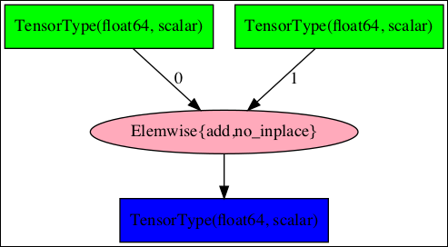
The complete program listing to generate the above image is given below −
from theano import *
a = tensor.dscalar()
b = tensor.dscalar()
c = a + b
f = theano.function([a,b], c)
theano.printing.pydotprint(f, outfile="scalar_addition.png", var_with_name_simple=True)
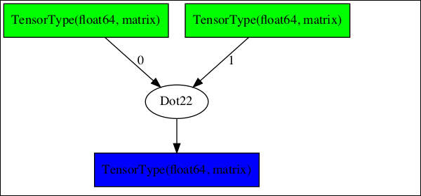
Symbolic Graph for Matrix Multiplier
Now, try creating the computation graph for our matrix multiplier. The complete listing for generating this graph is given below −
from theano import *
a = tensor.dmatrix()
b = tensor.dmatrix()
c = tensor.dot(a,b)
f = theano.function([a,b], c)
theano.printing.pydotprint(f, outfile="matrix_dot_product.png", var_with_name_simple=True)
The generated graph is shown here −
Complex Graphs
In larger expressions, the computational graphs could be very complex. One such graph taken from Theano documentation is shown here −
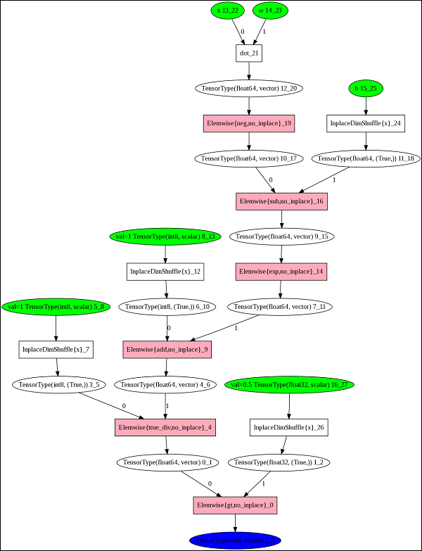
To understand the working of Theano, it is important to first know the significance of these computational graphs. With this understanding, we shall know the importance of Theano.
Why Theano?
By looking at the complexity of the computational graphs, you will now be able to understand the purpose behind developing Theano. A typical compiler would provide local optimizations in the program as it never looks at the entire computation as a single unit.
Theano implements very advanced optimization techniques to optimize the full computational graph. It combines the aspects of Algebra with aspects of an optimizing compiler. A part of the graph may be compiled into C-language code. For repeated calculations, the evaluation speed is critical and Theano meets this purpose by generating a very efficient code.
Theano - Data Types
Now, that you have understood the basics of Theano, let us begin with the different data types available to you for creating your expressions. The following table gives you a partial list of data types defined in Theano.
| Data type | Theano type |
|---|---|
| Byte | bscalar, bvector, bmatrix, brow, bcol, btensor3, btensor4, btensor5, btensor6, btensor7 |
| 16-bit integers | wscalar, wvector, wmatrix, wrow, wcol, wtensor3, wtensor4, wtensor5, wtensor6, wtensor7 |
| 32-bit integers | iscalar, ivector, imatrix, irow, icol, itensor3, itensor4, itensor5, itensor6, itensor7 |
| 64-bit integers | lscalar, lvector, lmatrix, lrow, lcol, ltensor3, ltensor4, ltensor5, ltensor6, ltensor7 |
| float | fscalar, fvector, fmatrix, frow, fcol, ftensor3, ftensor4, ftensor5, ftensor6, ftensor7 |
| double | dscalar, dvector, dmatrix, drow, dcol, dtensor3, dtensor4, dtensor5, dtensor6, dtensor7 |
| complex | cscalar, cvector, cmatrix, crow, ccol, ctensor3, ctensor4, ctensor5, ctensor6, ctensor7 |
The above list is not exhaustive and the reader is referred to the tensor creation document for a complete list.
I will now give you a few examples of how to create variables of various kinds of data in Theano.
Scalar
To construct a scalar variable you would use the syntax −
Syntax
x = theano.tensor.scalar ('x')
x = 5.0
print (x)
Output
5.0
One-dimensional Array
To create a one dimensional array, use the following declaration −
Example
f = theano.tensor.vector
f = (2.0, 5.0, 3.0)
print (f)f = theano.tensor.vector
f = (2.0, 5.0, 3.0)
print (f)
print (f[0])
print (f[2])
Output
(2.0, 5.0, 3.0)
2.0
3.0
If you do f[3] it would generate an index out of range error as shown here −
print f([3])
Output
IndexError                          Traceback (most recent call last)
<ipython-input-13-2a9c2a643c3a> in <module>
   4 print (f[0])
   5 print (f[2])
----> 6 print (f[3])
IndexError: tuple index out of range
Two-dimensional Array
To declare a two-dimensional array you would use the following code snippet −
Example
m = theano.tensor.matrix
m = ([2,3], [4,5], [2,4])
print (m[0])
print (m[1][0])
Output
[2, 3]
4
5-dimensional Array
To declare a 5-dimensional array, use the following syntax −
Example
m5 = theano.tensor.tensor5
m5 = ([0,1,2,3,4], [5,6,7,8,9], [10,11,12,13,14])
print (m5[1])
print (m5[2][3])
Output
[5, 6, 7, 8, 9]
13
You may declare a 3-dimensional array by using the data type tensor3 in place of tensor5, a 4-dimensional array using the data type tensor4, and so on up to tensor7.
Plural Constructors
Sometimes, you may want to create variables of the same type in a single declaration. You can do so by using the following syntax −
Syntax
from theano.tensor import * x, y, z = dmatrices('x', 'y', 'z')
x = ([1,2],[3,4],[5,6])
y = ([7,8],[9,10],[11,12])
z = ([13,14],[15,16],[17,18])
print (x[2])
print (y[1])
print (z[0])
Output
[5, 6]
[9, 10]
[13, 14]
Theano - Variables
In the previous chapter, while discussing the data types, we created and used Theano variables. To reiterate, we would use the following syntax to create a variable in Theano −
x = theano.tensor.fvector('x')
In this statement, we have created a variable x of type vector containing 32-bit floats. We are also naming it as x. The names are generally useful for debugging.
To declare a vector of 32-bit integers, you would use the following syntax −
i32 = theano.tensor.ivector
Here, we do not specify a name for the variable.
To declare a three-dimensional vector consisting of 64-bit floats, you would use the following declaration −
f64 = theano.tensor.dtensor3
The various types of constructors along with their data types are listed in the table below −
| Constructor | Data type | Dimensions |
|---|---|---|
| fvector | float32 | 1 |
| ivector | int32 | 1 |
| fscalar | float32 | 0 |
| fmatrix | float32 | 2 |
| ftensor3 | float32 | 3 |
| dtensor3 | float64 | 3 |
You may use a generic vector constructor and specify the data type explicitly as follows −
x = theano.tensor.vector ('x', dtype=int32)
In the next chapter, we will learn how to create shared variables.
Theano - Shared Variables
Many a times, you would need to create variables which are shared between different functions and also between multiple calls to the same function. To cite an example, while training a neural network you create weights vector for assigning a weight to each feature under consideration. This vector is modified on every iteration during the network training. Thus, it has to be globally accessible across the multiple calls to the same function. So we create a shared variable for this purpose. Typically, Theano moves such shared variables to the GPU, provided one is available. This speeds up the computation.
Syntax
You create a shared variable you use the following syntax −
import numpy
W = theano.shared(numpy.asarray([0.1, 0.25, 0.15, 0.3]), 'W')
Example
Here the NumPy array consisting of four floating point numbers is created. To set/get the W value you would use the following code snippet −
import numpy
W = theano.shared(numpy.asarray([0.1, 0.25, 0.15, 0.3]), 'W')
print ("Original: ", W.get_value())
print ("Setting new values (0.5, 0.2, 0.4, 0.2)")
W.set_value([0.5, 0.2, 0.4, 0.2])
print ("After modifications:", W.get_value())
Output
Original: [0.1 0.25 0.15 0.3 ]
Setting new values (0.5, 0.2, 0.4, 0.2)
After modifications: [0.5 0.2 0.4 0.2]
Theano - Functions
Theano function acts like a hook for interacting with the symbolic graph. A symbolic graph is compiled into a highly efficient execution code. It achieves this by restructuring mathematical equations to make them faster. It compiles some parts of the expression into C language code. It moves some tensors to the GPU, and so on.
The efficient compiled code is now given as an input to the Theano function. When you execute the Theano function, it assigns the result of computation to the variables specified by us. The type of optimization may be specified as FAST_COMPILE or FAST_RUN. This is specified in the environment variable THEANO_FLAGS.
A Theano function is declared using the following syntax −
f = theano.function ([x], y)
The first parameter [x] is the list of input variables and the second parameter y is the list of output variables.
Having now understood the basics of Theano, let us begin Theano coding with a trivial example.
Theano - Trivial Training Example
Theano is quite useful in training neural networks where we have to repeatedly calculate cost, and gradients to achieve an optimum. On large datasets, this becomes computationally intensive. Theano does this efficiently due to its internal optimizations of the computational graph that we have seen earlier.
Problem Statement
We shall now learn how to use Theano library to train a network. We will take a simple case where we start with a four feature dataset. We compute the sum of these features after applying a certain weight (importance) to each feature.
The goal of the training is to modify the weights assigned to each feature so that the sum reaches a target value of 100.
sum = f1 * w1 + f2 * w2 + f3 * w3 + f4 * w4
Where f1, f2, ... are the feature values and w1, w2, ... are the weights.
Let me quantize the example for a better understanding of the problem statement. We will assume an initial value of 1.0 for each feature and we will take w1 equals 0.1, w2 equals 0.25, w3 equals 0.15, and w4 equals 0.3. There is no definite logic in assigning the weight values, it is just our intuition. Thus, the initial sum is as follows −
sum = 1.0 * 0.1 + 1.0 * 0.25 + 1.0 * 0.15 + 1.0 * 0.3
Which sums to 0.8. Now, we will keep modifying the weight assignment so that this sum approaches 100. The current resultant value of 0.8 is far away from our desired target value of 100. In Machine Learning terms, we define cost as the difference between the target value minus the current output value, typically squared to blow up the error. We reduce this cost in each iteration by calculating the gradients and updating our weights vector.
Let us see how this entire logic is implemented in Theano.
Declaring Variables
We first declare our input vector x as follows −
x = tensor.fvector('x')
Where x is a single dimensional array of float values.
We define a scalar target variable as given below −
target = tensor.fscalar('target')
Next, we create a weights tensor W with the initial values as discussed above −
W = theano.shared(numpy.asarray([0.1, 0.25, 0.15, 0.3]), 'W')
Defining Theano Expression
We now calculate the output using the following expression −
y = (x * W).sum()
Note that in the above statement x and W are the vectors and not simple scalar variables. We now calculate the error (cost) with the following expression −
cost = tensor.sqr(target - y)
The cost is the difference between the target value and the current output, squared.
To calculate the gradient which tells us how far we are from the target, we use the built-in grad method as follows −
gradients = tensor.grad(cost, [W])
We now update the weights vector by taking a learning rate of 0.1 as follows −
W_updated = W - (0.1 * gradients[0])
Next, we need to update our weights vector using the above values. We do this in the following statement −
updates = [(W, W_updated)]
Defining/Invoking Theano Function
Lastly, we define a function in Theano to compute the sum.
f = function([x, target], y, updates=updates)
To invoke the above function a certain number of times, we create a for loop as follows −
for i in range(10):
output = f([1.0, 1.0, 1.0, 1.0], 100.0)
As said earlier, the input to the function is a vector containing the initial values for the four features - we assign the value of 1.0 to each feature without any specific reason. You may assign different values of your choice and check if the function ultimately converges. We will print the values of the weight vector and the corresponding output in each iteration. It is shown in the below code −
print ("iteration: ", i)
print ("Modified Weights: ", W.get_value())
print ("Output: ", output)
Full Program Listing
The complete program listing is reproduced here for your quick reference −
from theano import *
import numpy

x = tensor.fvector('x')
target = tensor.fscalar('target')

W = theano.shared(numpy.asarray([0.1, 0.25, 0.15, 0.3]), 'W')
print ("Weights: ", W.get_value())

y = (x * W).sum()
cost = tensor.sqr(target - y)
gradients = tensor.grad(cost, [W])
W_updated = W - (0.1 * gradients[0])
updates = [(W, W_updated)]

f = function([x, target], y, updates=updates)
for i in range(10):
   output = f([1.0, 1.0, 1.0, 1.0], 100.0)
   print ("iteration: ", i)
   print ("Modified Weights: ", W.get_value())
   print ("Output: ", output)
When you run the program you will see the following output −
Weights: [0.1 0.25 0.15 0.3 ]
iteration: 0
Modified Weights: [19.94 20.09 19.99 20.14]
Output: 0.8
iteration: 1
Modified Weights: [23.908 24.058 23.958 24.108]
Output: 80.16000000000001
iteration: 2
Modified Weights: [24.7016 24.8516 24.7516 24.9016]
Output: 96.03200000000001
iteration: 3
Modified Weights: [24.86032 25.01032 24.91032 25.06032]
Output: 99.2064
iteration: 4
Modified Weights: [24.892064 25.042064 24.942064 25.092064]
Output: 99.84128
iteration: 5
Modified Weights: [24.8984128 25.0484128 24.9484128 25.0984128]
Output: 99.968256
iteration: 6
Modified Weights: [24.89968256 25.04968256 24.94968256 25.09968256]
Output: 99.9936512
iteration: 7
Modified Weights: [24.89993651 25.04993651 24.94993651 25.09993651]
Output: 99.99873024
iteration: 8
Modified Weights: [24.8999873 25.0499873 24.9499873 25.0999873]
Output: 99.99974604799999
iteration: 9
Modified Weights: [24.89999746 25.04999746 24.94999746 25.09999746]
Output: 99.99994920960002
Observe that after four iterations, the output is 99.96 and after five iterations, it is 99.99, which is close to our desired target of 100.0.
Depending on the desired accuracy, you may safely conclude that the network is trained in 4 to 5 iterations. After the training completes, look up the weights vector, which after 5 iterations takes the following values −
iteration: 5
Modified Weights: [24.8984128 25.0484128 24.9484128 25.0984128]
You may now use these values in your network for deploying the model.
Theano - Conclusion
The Machine Learning model building involves intensive and repetitive computations involving tensors. These require intensive computing resources. As a regular compiler would provide the optimizations at the local level, it does not generally produce a fast execution code.
Theano first builds a computational graph for the entire computation. As the whole picture of computation is available as a single image during compilation, several optimization techniques can be applied during pre-compilation and thats what exactly Theano does. It restructures the computational graph, partly converts it into C, moves shared variables to GPU, and so on to generate a very fast executable code. The compiled code is then executed by a Theano function which just acts as a hook for injecting the compiled code into the runtime. Theano has proved its credentials and is widely accepted in both academics and industry.
