
Article Categories
- All Categories
-
 Data Structure
-
 Networking
-
 RDBMS
RDBMS
-
 Operating System
-
 Java
Java
-
 MS Excel
-
 iOS
iOS
-
 HTML
HTML
-
 CSS
CSS
-
 Android
-
 Python
-
 C Programming
-
 C++
C++
-
 C#
C#
-
 MongoDB
-
 MySQL
MySQL
-
 Javascript
-
 PHP
PHP
-
 Economics & Finance
Second Order System Transient Response
To understand the transient response of the second order system, consider the block diagram of closed loop system with unity negative feedback.
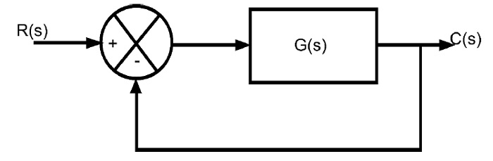
The open loop transfer function of the second order system is given by,
$$G(s)=\frac{\omega_{n}^{2}}{s(s+2\zeta\:\omega_{n})}$$
And the closed loop transfer function of the second order system is given by,
$$\frac{C(s)}{R(s)}=\frac{G(s)}{1+G(s)}=\frac{\omega_{n}^{2}}{s^{2}+2\zeta\:\omega_{n}s+\omega_{n}^{2}} \:\:\:\:...(1)$$
Where,
R(s) = Laplace transform of the input signal r(t),
C(s) = Laplace transform of the output signal c(t),
ξ= Damping Ration,
Ωn = Natrural frequency of oscillations.
As from the equation (1), we can see, the power of s is two in the denominator term. Thus, the transfer function represents a second order control system.
The characteristic equation of the second order system is given by equating the denominator of the closed loop transfer function to zero i.e.
$$s^{2}+2\zeta\:\omega_{n}s+\omega_{n}^{2}\:\:\:\:...(2)$$
The expression for the response of the second order system can be written as,
$$C(s)=(\frac{\omega_{n}^{2}}{s^{2}+2\zeta\:\omega_{n}s+\omega_{n}^{2}})R(s)\:\:\:\:\:...(3)$$
When ξ = 0, the system is Undamped.
When ξ = 1, the system is Critically damped.
When 0
When ξ > 1, the system is over damped.
Unit Step Response of Second Order System
Apply unit step signal at the input of the second order system,
$$r(t)=u(t)$$
Taking Laplace transform on the both sides
$$R(s)=\frac{1}{s}$$
Case 1 – When (ξ = 0) i.e., system is undamped, the equation (3) becomes,
$$C(s)=(\frac{\omega_{n}^{2}}{s^{2}+\omega_{n}^{2}})R(s)$$
$$\Rightarrow\:C(s)=(\frac{\omega_{n}^{2}}{s^{2}+\omega_{n}^{2}})(\frac{1}{s})=\frac{\omega_{n}^{2}}{s(s^{2}+\omega_{n}^{2})}$$
Taking the inverse Laplace transform on both the sides, we have,
$$C(t)=(1-\cos(\omega_{n}t))u(t)\:\:\:\:\:...(4)$$
The equation (4), shows that the unit step response of an undamped system is a continuous time signal of constant amplitude and frequency.
Case 2 – When (ξ = 1) i.e., system is critically damped, the equation (3) can be written as,
$$C(s)=(\frac{\omega_{n}^{2}}{s^{2}+2\omega_{n}s+\omega_{n}^{2}})R(s)=(\frac{\omega_{n}^{2}}{(s+\omega_{n})^{2}})R(s)$$
$$\Rightarrow\:C(s)=(\frac{\omega_{n}^{2}}{(s+\omega_{n})^{2}})\frac{1}{s}=(\frac{\omega_{n}^{2}}{s(s+\omega_{n})^{2}})$$
Finding the solution of the above equation by doing partial fraction, we get,
$$C(s)=\frac{1}{s}-\frac{1}{s+\omega_{n}}-\frac{\omega_{n}}{(s+\omega_{n})^{2}}$$
Taking the inverse Laplace transform on both the sides,
$$C(t)=(1-e^{-\omega_{n}t}-\omega_{n}te^{-\omega_{n}t})u(t)\:\:\:\:\:...(5)$$
When the system is critically damped then, the equation (5) shows, that the unit step response of the second order system would try to reach the steady state step input.
Case 3 – When (0
$$C(s)=(\frac{\omega_{n}^{2}}{(s+\zeta\:\omega_{n})^{2}+\omega_{n}^{2}(1-\zeta^{2})})R(s)$$
$$\Rightarrow\:C(s)=(\frac{\omega_{n}^{2}}{(s+\zeta\:\omega_{n})^{2}+\omega_{n}^{2}(1-\zeta^{2})})(\frac{1}{s})=\frac{\omega_{n}^{2}}{s((s+\zeta\:\omega_{n})^{2}+\omega_{n}^{2}(1-\zeta^{2}))}$$
Solving the above equation by partial fraction method, we get,
$$C(s)=\frac{1}{s}-\frac{(s+\zeta\:\omega_{n})}{(s+\zeta\:\omega_{n})^{2}+\omega_{d}^{2}}-\frac{\zeta}{\sqrt{1-\zeta^{2}}}(\frac{\omega_{d}}{(s+\zeta\:\omega_{n})^{2}+\omega_{d}^{2}})$$
Taking inverse Laplace on both the sides of the above equation, we get,
$$C(t)=(1-(\frac{e^{\zeta\:\omega_{n}t}}{\sqrt{1-\zeta^{2}}})\sin(\omega_{d}t+\theta))u(t)\:\:\:...(6)$$
Where,
$$\omega_{d}=\omega_{n}\sqrt{1-\zeta^{2}}$$
The equation (6) show, when the system is under damped then, the unit step response of the system is having damped oscillations i.e. response of decreasing amplitude.
Case 4 – When (ξ > 1) i.e., the system is over damped, the response expression can be written as,
$$C(s)=(\frac{\omega_{n}^{2}}{(s+\zeta\:\omega_{n})^{2}-\omega_{n}^{2}(\zeta^{2}-1)})R(s)$$
$$C(s)=(\frac{\omega_{n}^{2}}{(s+\zeta\:\omega_{n})^{2}-\omega_{n}^{2}(\zeta^{2}-1)})(\frac{1}{s})=\frac{\omega_{n}^{2}}{s((s+\zeta\:\omega_{n})^{2}-\omega_{n}^{2}(\zeta^{2}-1))}$$
$$C(s)=(\frac{\omega_{n}^{2}}{s(s+\zeta\:\omega_{n}+\omega_{n}\sqrt{\zeta^{2}-1})(s+\zeta\:\omega_{n}-\omega_{n}\sqrt{\zeta^{2}-1})})$$
By solving the above equation using the partial fraction method, we get,
$$C(s)=\frac{1}{s}+\frac{1}{2(\zeta\:+\sqrt{\zeta^{2}}-1)(\sqrt{\zeta^{2}}-1)}(\frac{1}{s+\zeta\:\omega_{n}+\omega_{n}\sqrt{\zeta^{2}-1}})-\frac{1}{2(\zeta\:-\sqrt{\zeta^{2}}-1)(\sqrt{\zeta^{2}}-1)}(\frac{1}{s+\zeta\:\omega_{n}-\omega_{n}\sqrt{\zeta^{2}-1}})$$
Taking inverse Laplace transform on both the sides,
$$C(t)=[1+\lbrace(\frac{1}{2(\zeta\:+\sqrt{\zeta^{2}-1})(\sqrt{\zeta^{2}-1})})e^{-(\zeta\:\omega_{n}+\omega_{n}\sqrt{\zeta^{2}-1})t}\rbrace\:-\:\lbrace(\frac{1}{2(\zeta\:-\sqrt{\zeta^{2}-1})(\sqrt{\zeta^{2}-1})})e^{-(\zeta\:\omega_{n}-\omega_{n}\sqrt{\zeta^{2}-1})t}\rbrace]u(t)\:\:\:\:\:...(7)$$
The equation (7) is the unit step response of the over damped second order system, the response will never reach steady state step input.
Unit Impulse Response of the Second Order System
Apply the unit impulse signal at the input of the second order system,
$$r(t)=\delta(t)$$
Taking Laplace transform on both the sides,
$$R(s)=1$$
As we know, the response of the second order system is given by,
$$c(s)=(\frac{\omega_{b}^{2}}{s^{2}+2\zeta\:\omega_{n}s+\omega_{n}^{2}})R(s)$$
Hence, for impulse input, we get,
$$c(s)=(\frac{\omega_{b}^{2}}{s^{2}+2\zeta\:\omega_{n}s+\omega_{n}^{2}})$$
Case 1 – Un-damped system (ξ = 0),
$$C(t)=\omega_{n}\sin(\omega_{n}t)\:\:\:\:for\:t\geq0\:\:\:\:\:\:....(8)$$
Case 2 – Critically damped system (ξ = 1),
$$C(s)=\omega_{n}^{2}te^{-\omega_{n}t}\:\:\:\:\:for\:t\geq0\:\:\:\:\:....(9)$$
Case 3 – Under damped system (0
$$C(t)=(\frac{\omega_{ne^{-\zeta\:\omega_{n}t}}}{\sqrt{1-\zeta^{2}}})\sin(\omega_{d}t)\:\:\:\:for\:t\geq0\:\:\:\:\:\:\:...(10)$$
Case 4 – Over damped system (ξ > 1),
$$C(t)=(\frac{\omega_{n}}{2\sqrt{1-\zeta^{2}}})[(e^{-(\zeta\:\omega_{n}-\omega_{n}\sqrt{\zeta^{2}-1})t})-(e^{-(\zeta\:\omega_{n}+\omega_{n}\sqrt{\zeta^{2}-1})t})]\:\:\:\:\:for\:t\geq0\:\:\:\:\:\:...(11)$$
Unit Ramp Response of the Second Order System
Apply a unit ramp signal at the input of a second order system,
$$r(t)=t\:u(t)$$
Taking Laplace transform on both the sides,
$$R(s)=\frac{1}{s^{2}}$$
The response equation of the second order system is given by,
$$C(s)=(\frac{\omega_{n}^{2}}{s^{2}+2\zeta\:\omega_{n}s+\omega_{n}^{2}})R(s)$$
With the applied ramp signal the above equation becomes,
$$C(s)=(\frac{\omega_{n}^{2}}{s^{2}+2\zeta\:\omega_{n}s+\omega_{n}^{2}})(\frac{1}{s^{2}})=(\frac{\omega_{n}^{2}}{s^{2}(s^{2}+2\zeta\:\omega_{n}s+\omega_{n}^{2})})$$
Hence, for an under damped system i.e. (0
$$C(t)=t-\frac{2\zeta}{\omega_{n}}+e^{-\zeta\:\omega_{n}t}(\frac{2\zeta}{\omega_{n}}\cos(\omega_{d}t)+\frac{2\zeta^{2}-1}{\omega_{n}\sqrt{1-\zeta^{2}}}\sin(\omega_{d}t))\:\:\:\:\:\:...(12)$$

7K+ Views
