- SciPy - Home
- SciPy - Introduction
- SciPy - Environment Setup
- SciPy - Basic Functionality
- SciPy - Relationship with NumPy
- SciPy Clusters
- SciPy - Clusters
- SciPy - Hierarchical Clustering
- SciPy - K-means Clustering
- SciPy - Distance Metrics
- SciPy Constants
- SciPy - Constants
- SciPy - Mathematical Constants
- SciPy - Physical Constants
- SciPy - Unit Conversion
- SciPy - Astronomical Constants
- SciPy - Fourier Transforms
- SciPy - FFTpack
- SciPy - Discrete Fourier Transform (DFT)
- SciPy - Fast Fourier Transform (FFT)
- SciPy Integration Equations
- SciPy - Integrate Module
- SciPy - Single Integration
- SciPy - Double Integration
- SciPy - Triple Integration
- SciPy - Multiple Integration
- SciPy Differential Equations
- SciPy - Differential Equations
- SciPy - Integration of Stochastic Differential Equations
- SciPy - Integration of Ordinary Differential Equations
- SciPy - Discontinuous Functions
- SciPy - Oscillatory Functions
- SciPy - Partial Differential Equations
- SciPy Interpolation
- SciPy - Interpolate
- SciPy - Linear 1-D Interpolation
- SciPy - Polynomial 1-D Interpolation
- SciPy - Spline 1-D Interpolation
- SciPy - Grid Data Multi-Dimensional Interpolation
- SciPy - RBF Multi-Dimensional Interpolation
- SciPy - Polynomial & Spline Interpolation
- SciPy Curve Fitting
- SciPy - Curve Fitting
- SciPy - Linear Curve Fitting
- SciPy - Non-Linear Curve Fitting
- SciPy - Input & Output
- SciPy - Input & Output
- SciPy - Reading & Writing Files
- SciPy - Working with Different File Formats
- SciPy - Efficient Data Storage with HDF5
- SciPy - Data Serialization
- SciPy Linear Algebra
- SciPy - Linalg
- SciPy - Matrix Creation & Basic Operations
- SciPy - Matrix LU Decomposition
- SciPy - Matrix QU Decomposition
- SciPy - Singular Value Decomposition
- SciPy - Cholesky Decomposition
- SciPy - Solving Linear Systems
- SciPy - Eigenvalues & Eigenvectors
- SciPy Image Processing
- SciPy - Ndimage
- SciPy - Reading & Writing Images
- SciPy - Image Transformation
- SciPy - Filtering & Edge Detection
- SciPy - Top Hat Filters
- SciPy - Morphological Filters
- SciPy - Low Pass Filters
- SciPy - High Pass Filters
- SciPy - Bilateral Filter
- SciPy - Median Filter
- SciPy - Non - Linear Filters in Image Processing
- SciPy - High Boost Filter
- SciPy - Laplacian Filter
- SciPy - Morphological Operations
- SciPy - Image Segmentation
- SciPy - Thresholding in Image Segmentation
- SciPy - Region-Based Segmentation
- SciPy - Connected Component Labeling
- SciPy Optimize
- SciPy - Optimize
- SciPy - Special Matrices & Functions
- SciPy - Unconstrained Optimization
- SciPy - Constrained Optimization
- SciPy - Matrix Norms
- SciPy - Sparse Matrix
- SciPy - Frobenius Norm
- SciPy - Spectral Norm
- SciPy Condition Numbers
- SciPy - Condition Numbers
- SciPy - Linear Least Squares
- SciPy - Non-Linear Least Squares
- SciPy - Finding Roots of Scalar Functions
- SciPy - Finding Roots of Multivariate Functions
- SciPy - Signal Processing
- SciPy - Signal Filtering & Smoothing
- SciPy - Short-Time Fourier Transform
- SciPy - Wavelet Transform
- SciPy - Continuous Wavelet Transform
- SciPy - Discrete Wavelet Transform
- SciPy - Wavelet Packet Transform
- SciPy - Multi-Resolution Analysis
- SciPy - Stationary Wavelet Transform
- SciPy - Statistical Functions
- SciPy - Stats
- SciPy - Descriptive Statistics
- SciPy - Continuous Probability Distributions
- SciPy - Discrete Probability Distributions
- SciPy - Statistical Tests & Inference
- SciPy - Generating Random Samples
- SciPy - Kaplan-Meier Estimator Survival Analysis
- SciPy - Cox Proportional Hazards Model Survival Analysis
- SciPy Spatial Data
- SciPy - Spatial
- SciPy - Special Functions
- SciPy - Special Package
- SciPy Advanced Topics
- SciPy - CSGraph
- SciPy - ODR
- SciPy Useful Resources
- SciPy - Reference
- SciPy - Quick Guide
- SciPy - Cheatsheet
- SciPy - Useful Resources
- SciPy - Discussion
SciPy - Quick Guide
SciPy - Introduction
SciPy, pronounced as Sigh Pi, is a scientific python open source, distributed under the BSD licensed library to perform Mathematical, Scientific and Engineering Computations.
The SciPy library depends on NumPy, which provides convenient and fast N-dimensional array manipulation. The SciPy library is built to work with NumPy arrays and provides many user-friendly and efficient numerical practices such as routines for numerical integration and optimization. Together, they run on all popular operating systems, are quick to install and are free of charge. NumPy and SciPy are easy to use, but powerful enough to depend on by some of the world's leading scientists and engineers.
SciPy Sub-packages
SciPy is organized into sub-packages covering different scientific computing domains. These are summarized in the following table −
| scipy.cluster | Vector quantization / Kmeans |
| scipy.constants | Physical and mathematical constants |
| scipy.fftpack | Fourier transform |
| scipy.integrate | Integration routines |
| scipy.interpolate | Interpolation |
| scipy.io | Data input and output |
| scipy.linalg | Linear algebra routines |
| scipy.ndimage | n-dimensional image package |
| scipy.odr | Orthogonal distance regression |
| scipy.optimize | Optimization |
| scipy.signal | Signal processing |
| scipy.sparse | Sparse matrices |
| scipy.spatial | Spatial data structures and algorithms |
| scipy.special | Any special mathematical functions |
| scipy.stats | Statistics |
Data Structure
The basic data structure used by SciPy is a multidimensional array provided by the NumPy module. NumPy provides some functions for Linear Algebra, Fourier Transforms and Random Number Generation, but not with the generality of the equivalent functions in SciPy.
SciPy - Environment Setup
Standard Python distribution does not come bundled with any SciPy module. A lightweight alternative is to install SciPy using the popular Python package installer,
pip install pandas
If we install the Anaconda Python package, Pandas will be installed by default. Following are the packages and links to install them in different operating systems.
Windows
Anaconda (from https://www.continuum.io) is a free Python distribution for the SciPy stack. It is also available for Linux and Mac.
Canopy (https://www.enthought.com/products/canopy/) is available free, as well as for commercial distribution with a full SciPy stack for Windows, Linux and Mac.
Python (x,y) − It is a free Python distribution with SciPy stack and Spyder IDE for Windows OS. (Downloadable from https://python-xy.github.io/)
Linux
Package managers of respective Linux distributions are used to install one or more packages in the SciPy stack.
Ubuntu
We can use the following path to install Python in Ubuntu.
sudo apt-get install python-numpy python-scipy
python-matplotlibipythonipython-notebook python-pandas python-sympy python-nose
Fedora
We can use the following path to install Python in Fedora.
sudo yum install numpyscipy python-matplotlibipython python-pandas
sympy python-nose atlas-devel
SciPy - Basic Functionality
By default, all the NumPy functions have been available through the SciPy namespace. There is no need to import the NumPy functions explicitly, when SciPy is imported. The main object of NumPy is the homogeneous multidimensional array. It is a table of elements (usually numbers), all of the same type, indexed by a tuple of positive integers. In NumPy, dimensions are called as axes. The number of axes is called as rank.
Now, let us revise the basic functionality of Vectors and Matrices in NumPy. As SciPy is built on top of NumPy arrays, understanding of NumPy basics is necessary. As most parts of linear algebra deals with matrices only.
NumPy Vector
A Vector can be created in multiple ways. Some of them are described below.
Converting Python array-like objects to NumPy
Let us consider the following example.
import numpy as np
list = [1,2,3,4]
arr = np.array(list)
print arr
The output of the above program will be as follows.
[1 2 3 4]
Intrinsic NumPy Array Creation
NumPy has built-in functions for creating arrays from scratch. Some of these functions are explained below.
Using zeros()
The zeros(shape) function will create an array filled with 0 values with the specified shape. The default dtype is float64. Let us consider the following example.
import numpy as np
print np.zeros((2, 3))
The output of the above program will be as follows.
array([[ 0., 0., 0.],
[ 0., 0., 0.]])
Using ones()
The ones(shape) function will create an array filled with 1 values. It is identical to zeros in all the other respects. Let us consider the following example.
import numpy as np
print np.ones((2, 3))
The output of the above program will be as follows.
array([[ 1., 1., 1.],
[ 1., 1., 1.]])
Using arange()
The arange() function will create arrays with regularly incrementing values. Let us consider the following example.
import numpy as np
print np.arange(7)
The above program will generate the following output.
array([0, 1, 2, 3, 4, 5, 6])
Defining the data type of the values
Let us consider the following example.
import numpy as np
arr = np.arange(2, 10, dtype = np.float)
print arr
print "Array Data Type :",arr.dtype
The above program will generate the following output.
[ 2. 3. 4. 5. 6. 7. 8. 9.]
Array Data Type : float64
Using linspace()
The linspace() function will create arrays with a specified number of elements, which will be spaced equally between the specified beginning and end values. Let us consider the following example.
import numpy as np
print np.linspace(1., 4., 6)
The above program will generate the following output.
array([ 1. , 1.6, 2.2, 2.8, 3.4, 4. ])
Matrix
A matrix is a specialized 2-D array that retains its 2-D nature through operations. It has certain special operators, such as * (matrix multiplication) and ** (matrix power). Let us consider the following example.
import numpy as np
print np.matrix('1 2; 3 4')
The above program will generate the following output.
matrix([[1, 2],
[3, 4]])
Conjugate Transpose of Matrix
This feature returns the (complex) conjugate transpose of self. Let us consider the following example.
import numpy as np
mat = np.matrix('1 2; 3 4')
print mat.H
The above program will generate the following output.
matrix([[1, 3],
        [2, 4]])
Transpose of Matrix
This feature returns the transpose of self. Let us consider the following example.
import numpy as np
mat = np.matrix('1 2; 3 4')
mat.T
The above program will generate the following output.
matrix([[1, 3],
        [2, 4]])
When we transpose a matrix, we make a new matrix whose rows are the columns of the original. A conjugate transposition, on the other hand, interchanges the row and the column index for each matrix element. The inverse of a matrix is a matrix that, if multiplied with the original matrix, results in an identity matrix.
SciPy - Cluster
K-means clustering is a method for finding clusters and cluster centers in a set of unlabelled data. Intuitively, we might think of a cluster as comprising of a group of data points, whose inter-point distances are small compared with the distances to points outside of the cluster. Given an initial set of K centers, the K-means algorithm iterates the following two steps −
For each center, the subset of training points (its cluster) that is closer to it is identified than any other center.
The mean of each feature for the data points in each cluster are computed, and this mean vector becomes the new center for that cluster.
These two steps are iterated until the centers no longer move or the assignments no longer change. Then, a new point x can be assigned to the cluster of the closest prototype. The SciPy library provides a good implementation of the K-Means algorithm through the cluster package. Let us understand how to use it.
K-Means Implementation in SciPy
We will understand how to implement K-Means in SciPy.
Import K-Means
We will see the implementation and usage of each imported function.
from SciPy.cluster.vq import kmeans,vq,whiten
Data generation
We have to simulate some data to explore the clustering.
from numpy import vstack,array
from numpy.random import rand

# data generation with three features
data = vstack((rand(100,3) + array([.5,.5,.5]),rand(100,3)))
Now, we have to check for data. The above program will generate the following output.
array([[ 1.48598868e+00, 8.17445796e-01, 1.00834051e+00],
       [ 8.45299768e-01, 1.35450732e+00, 8.66323621e-01],
       [ 1.27725864e+00, 1.00622682e+00, 8.43735610e-01],
       .
Normalize a group of observations on a per feature basis. Before running K-Means, it is beneficial to rescale each feature dimension of the observation set with whitening. Each feature is divided by its standard deviation across all observations to give it unit variance.
Whiten the data
We have to use the following code to whiten the data.
# whitening of data
data = whiten(data)
Compute K-Means with Three Clusters
Let us now compute K-Means with three clusters using the following code.
# computing K-Means with K = 3 (2 clusters)
centroids,_ = kmeans(data,3)
The above code performs K-Means on a set of observation vectors forming K clusters. The K-Means algorithm adjusts the centroids until sufficient progress cannot be made, i.e. the change in distortion, since the last iteration is less than some threshold. Here, we can observe the centroid of the cluster by printing the centroids variable using the code given below.
print(centroids)
The above code will generate the following output.
print(centroids)[ [ 2.26034702  1.43924335  1.3697022 ]
                  [ 2.63788572  2.81446462  2.85163854]
                  [ 0.73507256  1.30801855  1.44477558] ]
Assign each value to a cluster by using the code given below.
# assign each sample to a cluster
clx,_ = vq(data,centroids)
The vq function compares each observation vector in the M by N obs array with the centroids and assigns the observation to the closest cluster. It returns the cluster of each observation and the distortion. We can check the distortion as well. Let us check the cluster of each observation using the following code.
# check clusters of observation
print clx
The above code will generate the following output.
array([1, 1, 0, 1, 1, 1, 0, 1, 0, 0, 1, 1, 1, 0, 0, 1, 1, 0, 0, 1, 0, 2, 0, 2, 0, 1, 1, 1,
0, 0, 1, 1, 0, 0, 1, 1, 0, 0, 0, 0, 1, 1, 0, 0, 1, 1, 0, 0, 1, 0, 1, 0, 0, 0, 1, 1, 0, 0,
0, 1, 0, 1, 0, 0, 1, 0, 0, 0, 0, 0, 0, 0, 0, 0, 1, 0, 0, 1, 0, 0, 1, 0, 0, 0, 0, 0, 0, 0,
0, 1,  0, 0, 0, 0, 1, 0, 0, 1, 2, 1, 2, 2, 2, 2, 2, 2, 2, 2, 0, 2, 0, 2, 2, 2, 2, 2, 0, 0,
2, 2, 2, 1, 0, 2, 0, 2, 2, 2, 2, 2, 2, 2, 2, 2, 0, 2, 2, 1, 2, 2, 2, 2, 2, 2, 2, 2, 2, 2,
2, 2, 0, 2, 0, 2, 2, 2, 2, 2, 2, 2, 2, 2, 0, 2, 2, 2, 2, 0, 2, 2, 2, 2, 2, 2, 2, 2, 2, 2,
2, 2, 2, 2, 2, 2, 1, 2, 2, 2, 2, 2, 2, 2, 2, 2, 2, 2, 2, 2, 2, 2], dtype=int32)
The distinct values 0, 1, 2 of the above array indicate the clusters.
SciPy - Constants
SciPy constants package provides a wide range of constants, which are used in the general scientific area.
SciPy Constants Package
The scipy.constants package provides various constants. We have to import the required constant and use them as per the requirement. Let us see how these constant variables are imported and used.
To start with, let us compare the pi value by considering the following example.
#Import pi constant from both the packages
from scipy.constants import pi
from math import pi

print("sciPy - pi = %.16f"%scipy.constants.pi)
print("math - pi = %.16f"%math.pi)
The above program will generate the following output.
sciPy - pi = 3.1415926535897931
math - pi = 3.1415926535897931
List of Constants Available
The following tables describe in brief the various constants.
Mathematical Constants
| Sr. No. | Constant | Description |
|---|---|---|
| 1 | pi | pi |
| 2 | golden | Golden Ratio |
Physical Constants
The following table lists the most commonly used physical constants.
| Sr. No. | Constant & Description |
|---|---|
| 1 | c Speed of light in vacuum |
| 2 | speed_of_light Speed of light in vacuum |
| 3 | h Planck constant |
| 4 | Planck Planck constant h |
| 5 | G Newtons gravitational constant |
| 6 | e Elementary charge |
| 7 | R Molar gas constant |
| 8 | Avogadro Avogadro constant |
| 9 | k Boltzmann constant |
| 10 | electron_mass(OR) m_e Electronic mass |
| 11 | proton_mass (OR) m_p Proton mass |
| 12 | neutron_mass(OR)m_n Neutron mass |
Units
The following table has the list of SI units.
| Sr. No. | Unit | Value |
|---|---|---|
| 1 | milli | 0.001 |
| 2 | micro | 1e-06 |
| 3 | kilo | 1000 |
These units range from yotta, zetta, exa, peta, tera kilo, hector, nano, pico, to zepto.
Other Important Constants
The following table lists other important constants used in SciPy.
| Sr. No. | Unit | Value |
|---|---|---|
| 1 | gram | 0.001 kg |
| 2 | atomic mass | Atomic mass constant |
| 3 | degree | Degree in radians |
| 4 | minute | One minute in seconds |
| 5 | day | One day in seconds |
| 6 | inch | One inch in meters |
| 7 | micron | One micron in meters |
| 8 | light_year | One light-year in meters |
| 9 | atm | Standard atmosphere in pascals |
| 10 | acre | One acre in square meters |
| 11 | liter | One liter in cubic meters |
| 12 | gallon | One gallon in cubic meters |
| 13 | kmh | Kilometers per hour in meters per seconds |
| 14 | degree_Fahrenheit | One Fahrenheit in kelvins |
| 15 | eV | One electron volt in joules |
| 16 | hp | One horsepower in watts |
| 17 | dyn | One dyne in newtons |
| 18 | lambda2nu | Convert wavelength to optical frequency |
Remembering all of these are a bit tough. The easy way to get which key is for which function is with the scipy.constants.find() method. Let us consider the following example.
import scipy.constants
res = scipy.constants.physical_constants["alpha particle mass"]
print res
The above program will generate the following output.
[
   'alpha particle mass',
   'alpha particle mass energy equivalent',
   'alpha particle mass energy equivalent in MeV',
   'alpha particle mass in u',
   'electron to alpha particle mass ratio'
]
This method returns the list of keys, else nothing if the keyword does not match.
SciPy - FFTpack
Fourier Transformation is computed on a time domain signal to check its behavior in the frequency domain. Fourier transformation finds its application in disciplines such as signal and noise processing, image processing, audio signal processing, etc. SciPy offers the fftpack module, which lets the user compute fast Fourier transforms.
Following is an example of a sine function, which will be used to calculate Fourier transform using the fftpack module.
Fast Fourier Transform
Let us understand what fast Fourier transform is in detail.
One Dimensional Discrete Fourier Transform
The FFT y[k] of length N of the length-N sequence x[n] is calculated by fft() and the inverse transform is calculated using ifft(). Let us consider the following example
#Importing the fft and inverse fft functions from fftpackage
from scipy.fftpack import fft

#create an array with random n numbers
x = np.array([1.0, 2.0, 1.0, -1.0, 1.5])

#Applying the fft function
y = fft(x)
print y
The above program will generate the following output.
[ 4.50000000+0.j           2.08155948-1.65109876j   -1.83155948+1.60822041j
 -1.83155948-1.60822041j   2.08155948+1.65109876j ]
Let us look at another example
#FFT is already in the workspace, using the same workspace to for inverse transform

yinv = ifft(y)

print yinv
The above program will generate the following output.
[ 1.0+0.j 2.0+0.j 1.0+0.j -1.0+0.j 1.5+0.j ]
The scipy.fftpack module allows computing fast Fourier transforms. As an illustration, a (noisy) input signal may look as follows −
import numpy as np
time_step = 0.02
period = 5.
time_vec = np.arange(0, 20, time_step)
sig = np.sin(2 * np.pi / period * time_vec) + 0.5 *np.random.randn(time_vec.size)
print sig.size
We are creating a signal with a time step of 0.02 seconds. The last statement prints the size of the signal sig. The output would be as follows −
1000
We do not know the signal frequency; we only know the sampling time step of the signal sig. The signal is supposed to come from a real function, so the Fourier transform will be symmetric. The scipy.fftpack.fftfreq() function will generate the sampling frequencies and scipy.fftpack.fft() will compute the fast Fourier transform.
Let us understand this with the help of an example.
from scipy import fftpack
sample_freq = fftpack.fftfreq(sig.size, d = time_step)
sig_fft = fftpack.fft(sig)
print sig_fft
The above program will generate the following output.
array([
   25.45122234 +0.00000000e+00j,   6.29800973 +2.20269471e+00j,
   11.52137858 -2.00515732e+01j,   1.08111300 +1.35488579e+01j,
   .])
Discrete Cosine Transform
A Discrete Cosine Transform (DCT) expresses a finite sequence of data points in terms of a sum of cosine functions oscillating at different frequencies. SciPy provides a DCT with the function dct and a corresponding IDCT with the function idct. Let us consider the following example.
from scipy.fftpack import dct
print dct(np.array([4., 3., 5., 10., 5., 3.]))
The above program will generate the following output.
array([ 60., -3.48476592, -13.85640646, 11.3137085, 6., -6.31319305])
The inverse discrete cosine transform reconstructs a sequence from its discrete cosine transform (DCT) coefficients. The idct function is the inverse of the dct function. Let us understand this with the following example.
from scipy.fftpack import dct
print idct(np.array([4., 3., 5., 10., 5., 3.]))
The above program will generate the following output.
array([ 39.15085889, -20.14213562, -6.45392043, 7.13341236,
8.14213562, -3.83035081])
SciPy - Integrate
When a function cannot be integrated analytically, or is very difficult to integrate analytically, one generally turns to numerical integration methods. SciPy has a number of routines for performing numerical integration. Most of them are found in the same scipy.integrate library. The following table lists some commonly used functions.
| Sr No. | Function & Description |
|---|---|
| 1 | quad Single integration |
| 2 | dblquad Double integration |
| 3 | tplquad Triple integration |
| 4 | nquad n-fold multiple integration |
| 5 | fixed_quad Gaussian quadrature, order n |
| 6 | quadrature Gaussian quadrature to tolerance |
| 7 | romberg Romberg integration |
| 8 | trapz Trapezoidal rule |
| 9 | cumtrapz Trapezoidal rule to cumulatively compute integral |
| 10 | simps Simpsons rule |
| 11 | romb Romberg integration |
| 12 | polyint Analytical polynomial integration (NumPy) |
| 13 | poly1d Helper function for polyint (NumPy) |
Single Integrals
The Quad function is the workhorse of SciPys integration functions. Numerical integration is sometimes called quadrature, hence the name. It is normally the default choice for performing single integrals of a function f(x) over a given fixed range from a to b.
$$\int_{a}^{b} f(x)dx$$
The general form of quad is scipy.integrate.quad(f, a, b), Where f is the name of the function to be integrated. Whereas, a and b are the lower and upper limits, respectively. Let us see an example of the Gaussian function, integrated over a range of 0 and 1.
We first need to define the function → $f(x) = e^{-x^2}$ , this can be done using a lambda expression and then call the quad method on that function.
import scipy.integrate
from numpy import exp
f= lambda x:exp(-x**2)
i = scipy.integrate.quad(f, 0, 1)
print i
The above program will generate the following output.
(0.7468241328124271, 8.291413475940725e-15)
The quad function returns the two values, in which the first number is the value of integral and the second value is the estimate of the absolute error in the value of integral.
Note − Since quad requires the function as the first argument, we cannot directly pass exp as the argument. The Quad function accepts positive and negative infinity as limits. The Quad function can integrate standard predefined NumPy functions of a single variable, such as exp, sin and cos.
Multiple Integrals
The mechanics for double and triple integration have been wrapped up into the functions dblquad, tplquad and nquad. These functions integrate four or six arguments, respectively. The limits of all inner integrals need to be defined as functions.
Double Integrals
The general form of dblquad is scipy.integrate.dblquad(func, a, b, gfun, hfun). Where, func is the name of the function to be integrated, a and b are the lower and upper limits of the x variable, respectively, while gfun and hfun are the names of the functions that define the lower and upper limits of the y variable.
As an example, let us perform the double integral method.
$$\int_{0}^{1/2} dy \int_{0}^{\sqrt{1-4y^2}} 16xy \:dx$$
We define the functions f, g, and h, using the lambda expressions. Note that even if g and h are constants, as they may be in many cases, they must be defined as functions, as we have done here for the lower limit.
import scipy.integrate
from numpy import exp
from math import sqrt
f = lambda x, y : 16*x*y
g = lambda x : 0
h = lambda y : sqrt(1-4*y**2)
i = scipy.integrate.dblquad(f, 0, 0.5, g, h)
print i
The above program will generate the following output.
(0.5, 1.7092350012594845e-14)
In addition to the routines described above, scipy.integrate has a number of other integration routines, including nquad, which performs n-fold multiple integration, as well as other routines that implement various integration algorithms. However, quad and dblquad will meet most of our needs for numerical integration.
SciPy - Interpolate
In this chapter, we will discuss how interpolation helps in SciPy.
What is Interpolation?
Interpolation is the process of finding a value between two points on a line or a curve. To help us remember what it means, we should think of the first part of the word, 'inter,' as meaning 'enter,' which reminds us to look 'inside' the data we originally had. This tool, interpolation, is not only useful in statistics, but is also useful in science, business, or when there is a need to predict values that fall within two existing data points.
Let us create some data and see how this interpolation can be done using the scipy.interpolate package.
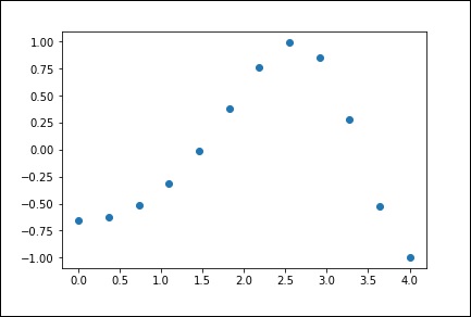
import numpy as np
from scipy import interpolate
import matplotlib.pyplot as plt
x = np.linspace(0, 4, 12)
y = np.cos(x**2/3+4)
print x,y
The above program will generate the following output.
(
   array([0.,  0.36363636,  0.72727273,  1.09090909,  1.45454545, 1.81818182,
          2.18181818,  2.54545455,  2.90909091,  3.27272727,  3.63636364,  4.]),

   array([-0.65364362,  -0.61966189,  -0.51077021,  -0.31047698,  -0.00715476,
           0.37976236,   0.76715099,   0.99239518,   0.85886263,   0.27994201,
          -0.52586509,  -0.99582185])
)
Now, we have two arrays. Assuming those two arrays as the two dimensions of the points in space, let us plot using the following program and see how they look like.
plt.plot(x, y,o)
plt.show()
The above program will generate the following output.
1-D Interpolation
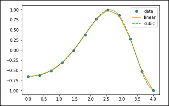
The interp1d class in the scipy.interpolate is a convenient method to create a function based on fixed data points, which can be evaluated anywhere within the domain defined by the given data using linear interpolation.
By using the above data, let us create a interpolate function and draw a new interpolated graph.
f1 = interp1d(x, y,kind = 'linear')

f2 = interp1d(x, y, kind = 'cubic')
Using the interp1d function, we created two functions f1 and f2. These functions, for a given input x returns y. The third variable kind represents the type of the interpolation technique. 'Linear', 'Nearest', 'Zero', 'Slinear', 'Quadratic', 'Cubic' are a few techniques of interpolation.
Now, let us create a new input of more length to see the clear difference of interpolation. We will use the same function of the old data on the new data.
xnew = np.linspace(0, 4,30)

plt.plot(x, y, 'o', xnew, f(xnew), '-', xnew, f2(xnew), '--')

plt.legend(['data', 'linear', 'cubic','nearest'], loc = 'best')

plt.show()
The above program will generate the following output.
Splines
To draw smooth curves through data points, drafters once used thin flexible strips of wood, hard rubber, metal or plastic called mechanical splines. To use a mechanical spline, pins were placed at a judicious selection of points along a curve in a design, and then the spline was bent, so that it touched each of these pins.
Clearly, with this construction, the spline interpolates the curve at these pins. It can be used to reproduce the curve in other drawings. The points where the pins are located is called knots. We can change the shape of the curve defined by the spline by adjusting the location of the knots.
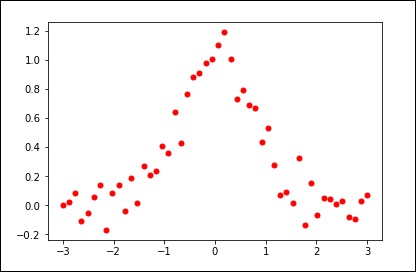
Univariate Spline
One-dimensional smoothing spline fits a given set of data points. The UnivariateSpline class in scipy.interpolate is a convenient method to create a function, based on fixed data points class scipy.interpolate.UnivariateSpline(x, y, w = None, bbox = [None, None], k = 3, s = None, ext = 0, check_finite = False).
Parameters − Following are the parameters of a Univariate Spline.
This fits a spline y = spl(x) of degree k to the provided x, y data.
w − Specifies the weights for spline fitting. Must be positive. If none (default), weights are all equal.
s − Specifies the number of knots by specifying a smoothing condition.
k − Degree of the smoothing spline. Must be <= 5. Default is k = 3, a cubic spline.
Ext − Controls the extrapolation mode for elements not in the interval defined by the knot sequence.
if ext = 0 or extrapolate, returns the extrapolated value.
if ext = 1 or zero, returns 0
if ext = 2 or raise, raises a ValueError
if ext = 3 of const, returns the boundary value.
check_finite Whether to check that the input arrays contain only finite numbers.
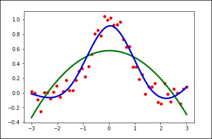
Let us consider the following example.
import matplotlib.pyplot as plt
from scipy.interpolate import UnivariateSpline
x = np.linspace(-3, 3, 50)
y = np.exp(-x**2) + 0.1 * np.random.randn(50)
plt.plot(x, y, 'ro', ms = 5)
plt.show()
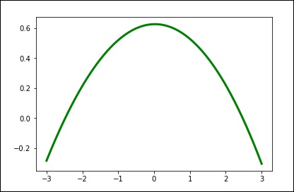
Use the default value for the smoothing parameter.
spl = UnivariateSpline(x, y)
xs = np.linspace(-3, 3, 1000)
plt.plot(xs, spl(xs), 'g', lw = 3)
plt.show()
Manually change the amount of smoothing.
spl.set_smoothing_factor(0.5)
plt.plot(xs, spl(xs), 'b', lw = 3)
plt.show()
SciPy - Input & Output
The Scipy.io (Input and Output) package provides a wide range of functions to work around with different format of files. Some of these formats are −
- Matlab
- IDL
- Matrix Market
- Wave
- Arff
- Netcdf, etc.
Let us discuss in detail about the most commonly used file formats −
MATLAB
Following are the functions used to load and save a .mat file.
| Sr. No. | Function & Description |
|---|---|
| 1 | loadmat Loads a MATLAB file |
| 2 | savemat Saves a MATLAB file |
| 3 | whosmat Lists variables inside a MATLAB file |
Let us consider the following example.
import scipy.io as sio
import numpy as np

#Save a mat file
vect = np.arange(10)
sio.savemat('array.mat', {'vect':vect})

#Now Load the File
mat_file_content = sio.loadmat(array.mat)
Print mat_file_content
The above program will generate the following output.
{
   'vect': array([[0, 1, 2, 3, 4, 5, 6, 7, 8, 9]]), '__version__': '1.0',
   '__header__': 'MATLAB 5.0 MAT-file Platform: posix, Created on: Sat Sep 30
   09:49:32 2017', '__globals__': []
}
We can see the array along with the Meta information. If we want to inspect the contents of a MATLAB file without reading the data into memory, use the whosmat command as shown below.
import scipy.io as sio
mat_file_content = sio.whosmat(array.mat)
print mat_file_content
The above program will generate the following output.
[('vect', (1, 10), 'int64')]
SciPy - Linalg
SciPy is built using the optimized ATLAS LAPACK and BLAS libraries. It has very fast linear algebra capabilities. All of these linear algebra routines expect an object that can be converted into a two-dimensional array. The output of these routines is also a two-dimensional array.
SciPy.linalg vs NumPy.linalg
A scipy.linalg contains all the functions that are in numpy.linalg. Additionally, scipy.linalg also has some other advanced functions that are not in numpy.linalg. Another advantage of using scipy.linalg over numpy.linalg is that it is always compiled with BLAS/LAPACK support, while for NumPy this is optional. Therefore, the SciPy version might be faster depending on how NumPy was installed.
Linear Equations
The scipy.linalg.solve feature solves the linear equation a * x + b * y = Z, for the unknown x, y values.
As an example, assume that it is desired to solve the following simultaneous equations.
x + 3y + 5z = 10
2x + 5y + z = 8
2x + 3y + 8z = 3
To solve the above equation for the x, y, z values, we can find the solution vector using a matrix inverse as shown below.
$$\begin{bmatrix} x\\ y\\ z \end{bmatrix} = \begin{bmatrix} 1 & 3 & 5\\ 2 & 5 & 1\\ 2 & 3 & 8 \end{bmatrix}^{-1} \begin{bmatrix} 10\\ 8\\ 3 \end{bmatrix} = \frac{1}{25} \begin{bmatrix} -232\\ 129\\ 19 \end{bmatrix} = \begin{bmatrix} -9.28\\ 5.16\\ 0.76 \end{bmatrix}.$$
However, it is better to use the linalg.solve command, which can be faster and more numerically stable.
The solve function takes two inputs a and b in which a represents the coefficients and b represents the respective right hand side value and returns the solution array.
Let us consider the following example.
#importing the scipy and numpy packages
from scipy import linalg
import numpy as np

#Declaring the numpy arrays
a = np.array([[3, 2, 0], [1, -1, 0], [0, 5, 1]])
b = np.array([2, 4, -1])

#Passing the values to the solve function
x = linalg.solve(a, b)

#printing the result array
print x
The above program will generate the following output.
array([ 2., -2., 9.])
Finding a Determinant
The determinant of a square matrix A is often denoted as |A| and is a quantity often used in linear algebra. In SciPy, this is computed using the det() function. It takes a matrix as input and returns a scalar value.
Let us consider the following example.
#importing the scipy and numpy packages
from scipy import linalg
import numpy as np

#Declaring the numpy array
A = np.array([[1,2],[3,4]])

#Passing the values to the det function
x = linalg.det(A)

#printing the result
print x
The above program will generate the following output.
-2.0
Eigenvalues and Eigenvectors
The eigenvalue-eigenvector problem is one of the most commonly employed linear algebra operations. We can find the Eigen values () and the corresponding Eigen vectors (v) of a square matrix (A) by considering the following relation −
Av = v
scipy.linalg.eig computes the eigenvalues from an ordinary or generalized eigenvalue problem. This function returns the Eigen values and the Eigen vectors.
Let us consider the following example.
#importing the scipy and numpy packages
from scipy import linalg
import numpy as np

#Declaring the numpy array
A = np.array([[1,2],[3,4]])

#Passing the values to the eig function
l, v = linalg.eig(A)

#printing the result for eigen values
print l

#printing the result for eigen vectors
print v
The above program will generate the following output.
array([-0.37228132+0.j, 5.37228132+0.j]) #--Eigen Values
array([[-0.82456484, -0.41597356], #--Eigen Vectors
       [ 0.56576746, -0.90937671]])
Singular Value Decomposition
A Singular Value Decomposition (SVD) can be thought of as an extension of the eigenvalue problem to matrices that are not square.
The scipy.linalg.svd factorizes the matrix a into two unitary matrices U and Vh and a 1-D array s of singular values (real, non-negative) such that a == U*S*Vh, where S is a suitably shaped matrix of zeros with the main diagonal s.
Let us consider the following example.
#importing the scipy and numpy packages
from scipy import linalg
import numpy as np

#Declaring the numpy array
a = np.random.randn(3, 2) + 1.j*np.random.randn(3, 2)

#Passing the values to the eig function
U, s, Vh = linalg.svd(a)

# printing the result
print U, Vh, s
The above program will generate the following output.
(
   array([
      [ 0.54828424-0.23329795j, -0.38465728+0.01566714j,
      -0.18764355+0.67936712j],
      [-0.27123194-0.5327436j , -0.57080163-0.00266155j,
      -0.39868941-0.39729416j],
      [ 0.34443818+0.4110186j , -0.47972716+0.54390586j,
      0.25028608-0.35186815j]
   ]),

   array([ 3.25745379, 1.16150607]),

   array([
      [-0.35312444+0.j , 0.32400401+0.87768134j],
      [-0.93557636+0.j , -0.12229224-0.33127251j]
   ])
)
SciPy - Ndimage
The SciPy ndimage submodule is dedicated to image processing. Here, ndimage means an n-dimensional image.
Some of the most common tasks in image processing are as follows &miuns;
- Input/Output, displaying images
- Basic manipulations − Cropping, flipping, rotating, etc.
- Image filtering − De-noising, sharpening, etc.
- Image segmentation − Labeling pixels corresponding to different objects
- Classification
- Feature extraction
- Registration
Let us discuss how some of these can be achieved using SciPy.
Opening and Writing to Image Files
The misc package in SciPy comes with some images. We use those images to learn the image manipulations. Let us consider the following example.
from scipy import misc
f = misc.face()
misc.imsave('face.png', f) # uses the Image module (PIL)

import matplotlib.pyplot as plt
plt.imshow(f)
plt.show()
The above program will generate the following output.
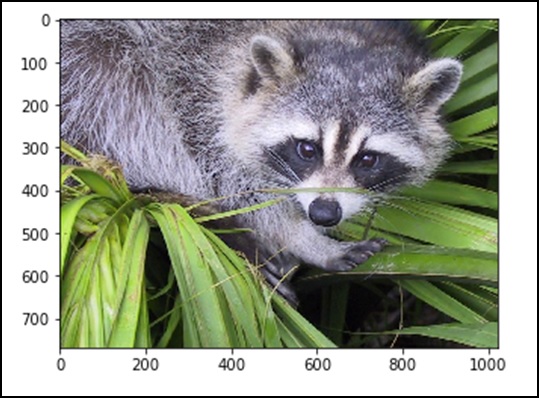
Any images in its raw format is the combination of colors represented by the numbers in the matrix format. A machine understands and manipulates the images based on those numbers only. RGB is a popular way of representation.
Let us see the statistical information of the above image.
from scipy import misc
face = misc.face(gray = False)
print face.mean(), face.max(), face.min()
The above program will generate the following output.
110.16274388631184, 255, 0
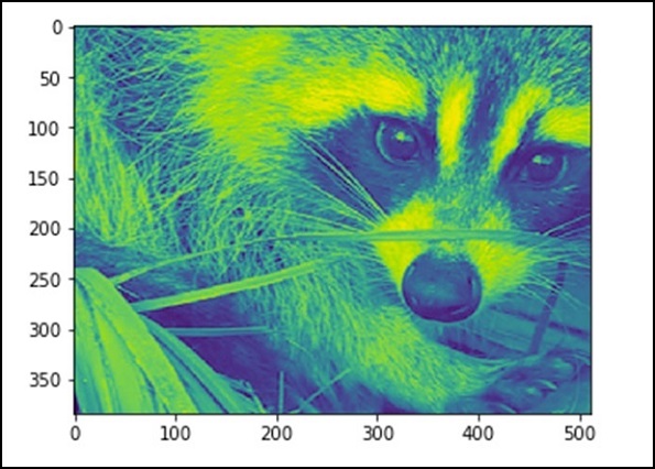
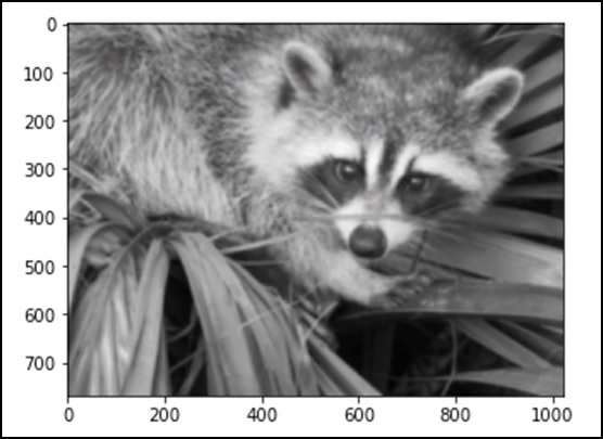
Now, we know that the image is made out of numbers, so any change in the value of the number alters the original image. Let us perform some geometric transformations on the image. The basic geometric operation is cropping
from scipy import misc
face = misc.face(gray = True)
lx, ly = face.shape
# Cropping
crop_face = face[lx / 4: - lx / 4, ly / 4: - ly / 4]
import matplotlib.pyplot as plt
plt.imshow(crop_face)
plt.show()
The above program will generate the following output.
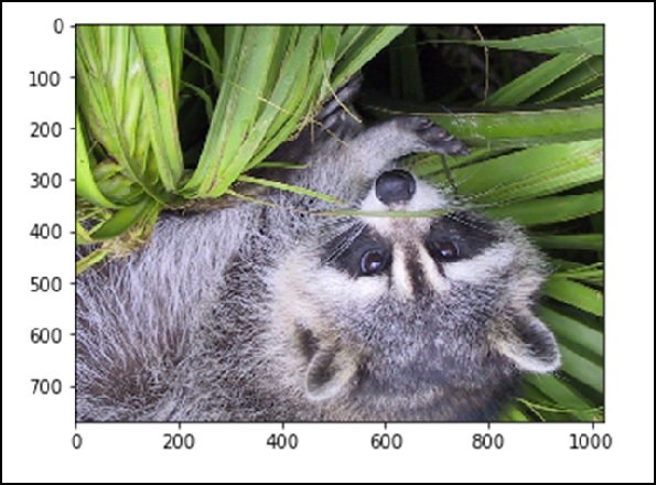
We can also perform some basic operations such as turning the image upside down as described below.
# up <-> down flip
from scipy import misc
face = misc.face()
flip_ud_face = np.flipud(face)

import matplotlib.pyplot as plt
plt.imshow(flip_ud_face)
plt.show()
The above program will generate the following output.
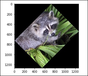
Besides this, we have the rotate() function, which rotates the image with a specified angle.
# rotation
from scipy import misc,ndimage
face = misc.face()
rotate_face = ndimage.rotate(face, 45)

import matplotlib.pyplot as plt
plt.imshow(rotate_face)
plt.show()
The above program will generate the following output.
Filters
Let us discuss how filters help in image processing.
What is filtering in image processing?
Filtering is a technique for modifying or enhancing an image. For example, you can filter an image to emphasize certain features or remove other features. Image processing operations implemented with filtering include Smoothing, Sharpening, and Edge Enhancement.
Filtering is a neighborhood operation, in which the value of any given pixel in the output image is determined by applying some algorithm to the values of the pixels in the neighborhood of the corresponding input pixel. Let us now perform a few operations using SciPy ndimage.
Blurring
Blurring is widely used to reduce the noise in the image. We can perform a filter operation and see the change in the image. Let us consider the following example.
from scipy import misc
face = misc.face()
blurred_face = ndimage.gaussian_filter(face, sigma=3)
import matplotlib.pyplot as plt
plt.imshow(blurred_face)
plt.show()
The above program will generate the following output.
The sigma value indicates the level of blur on a scale of five. We can see the change on the image quality by tuning the sigma value. For more details of blurring, click on → DIP (Digital Image Processing) Tutorial.
Edge Detection
Let us discuss how edge detection helps in image processing.
What is Edge Detection?
Edge detection is an image processing technique for finding the boundaries of objects within images. It works by detecting discontinuities in brightness. Edge detection is used for image segmentation and data extraction in areas such as Image Processing, Computer Vision and Machine Vision.
The most commonly used edge detection algorithms include
- Sobel
- Canny
- Prewitt
- Roberts
- Fuzzy Logic methods
Let us consider the following example.
import scipy.ndimage as nd
import numpy as np

im = np.zeros((256, 256))
im[64:-64, 64:-64] = 1
im[90:-90,90:-90] = 2
im = ndimage.gaussian_filter(im, 8)

import matplotlib.pyplot as plt
plt.imshow(im)
plt.show()
The above program will generate the following output.
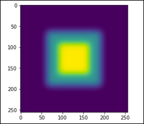
The image looks like a square block of colors. Now, we will detect the edges of those colored blocks. Here, ndimage provides a function called Sobel to carry out this operation. Whereas, NumPy provides the Hypot function to combine the two resultant matrices to one.
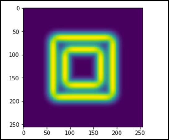
Let us consider the following example.
import scipy.ndimage as nd
import matplotlib.pyplot as plt

im = np.zeros((256, 256))
im[64:-64, 64:-64] = 1
im[90:-90,90:-90] = 2
im = ndimage.gaussian_filter(im, 8)

sx = ndimage.sobel(im, axis = 0, mode = 'constant')
sy = ndimage.sobel(im, axis = 1, mode = 'constant')
sob = np.hypot(sx, sy)

plt.imshow(sob)
plt.show()
The above program will generate the following output.
SciPy - Optimize
The scipy.optimize package provides several commonly used optimization algorithms. This module contains the following aspects −
Unconstrained and constrained minimization of multivariate scalar functions (minimize()) using a variety of algorithms (e.g. BFGS, Nelder-Mead simplex, Newton Conjugate Gradient, COBYLA or SLSQP)
Global (brute-force) optimization routines (e.g., anneal(), basinhopping())
Least-squares minimization (leastsq()) and curve fitting (curve_fit()) algorithms
Scalar univariate functions minimizers (minimize_scalar()) and root finders (newton())
Multivariate equation system solvers (root()) using a variety of algorithms (e.g. hybrid Powell, Levenberg-Marquardt or large-scale methods such as Newton-Krylov)
Unconstrained & Constrained minimization of multivariate scalar functions
The minimize() function provides a common interface to unconstrained and constrained minimization algorithms for multivariate scalar functions in scipy.optimize. To demonstrate the minimization function, consider the problem of minimizing the Rosenbrock function of the NN variables −
$$f(x) = \sum_{i = 1}^{N-1} \:100(x_i - x_{i-1}^{2})$$
The minimum value of this function is 0, which is achieved when xi = 1.
NelderMead Simplex Algorithm
In the following example, the minimize() routine is used with the Nelder-Mead simplex algorithm (method = 'Nelder-Mead') (selected through the method parameter). Let us consider the following example.
import numpy as np
from scipy.optimize import minimize

def rosen(x):

x0 = np.array([1.3, 0.7, 0.8, 1.9, 1.2])
res = minimize(rosen, x0, method='nelder-mead')

print(res.x)
The above program will generate the following output.
[7.93700741e+54 -5.41692163e+53 6.28769150e+53 1.38050484e+55 -4.14751333e+54]
The simplex algorithm is probably the simplest way to minimize a fairly well-behaved function. It requires only function evaluations and is a good choice for simple minimization problems. However, because it does not use any gradient evaluations, it may take longer to find the minimum.
Another optimization algorithm that needs only function calls to find the minimum is the Powells method, which is available by setting method = 'powell' in the minimize() function.
Least Squares
Solve a nonlinear least-squares problem with bounds on the variables. Given the residuals f(x) (an m-dimensional real function of n real variables) and the loss function rho(s) (a scalar function), least_squares find a local minimum of the cost function F(x). Let us consider the following example.
In this example, we find a minimum of the Rosenbrock function without bounds on the independent variables.
#Rosenbrock Function
def fun_rosenbrock(x):
   return np.array([10 * (x[1] - x[0]**2), (1 - x[0])])

from scipy.optimize import least_squares
input = np.array([2, 2])
res = least_squares(fun_rosenbrock, input)

print res
Notice that, we only provide the vector of the residuals. The algorithm constructs the cost function as a sum of squares of the residuals, which gives the Rosenbrock function. The exact minimum is at x = [1.0,1.0].
The above program will generate the following output.
active_mask: array([ 0., 0.])
      cost: 9.8669242910846867e-30
      fun: array([ 4.44089210e-15, 1.11022302e-16])
      grad: array([ -8.89288649e-14, 4.44089210e-14])
      jac: array([[-20.00000015,10.],[ -1.,0.]])
   message: '`gtol` termination condition is satisfied.'
      nfev: 3
      njev: 3
   optimality: 8.8928864934219529e-14
      status: 1
      success: True
         x: array([ 1., 1.])
Root finding
Let us understand how root finding helps in SciPy.
Scalar functions
If one has a single-variable equation, there are four different root-finding algorithms, which can be tried. Each of these algorithms require the endpoints of an interval in which a root is expected (because the function changes signs). In general, brentq is the best choice, but the other methods may be useful in certain circumstances or for academic purposes.
Fixed-point solving
A problem closely related to finding the zeros of a function is the problem of finding a fixed point of a function. A fixed point of a function is the point at which evaluation of the function returns the point: g(x) = x. Clearly the fixed point of gg is the root of f(x) = g(x)x. Equivalently, the root of ff is the fixed_point of g(x) = f(x)+x. The routine fixed_point provides a simple iterative method using the Aitkens sequence acceleration to estimate the fixed point of gg, if a starting point is given.
Sets of equations
Finding a root of a set of non-linear equations can be achieved using the root() function. Several methods are available, amongst which hybr (the default) and lm, respectively use the hybrid method of Powell and the Levenberg-Marquardt method from the MINPACK.
The following example considers the single-variable transcendental equation.
x2 + 2cos(x) = 0
A root of which can be found as follows −
import numpy as np
from scipy.optimize import root
def func(x):
   return x*2 + 2 * np.cos(x)
sol = root(func, 0.3)
print sol
The above program will generate the following output.
fjac: array([[-1.]])
fun: array([ 2.22044605e-16])
message: 'The solution converged.'
   nfev: 10
   qtf: array([ -2.77644574e-12])
      r: array([-3.34722409])
   status: 1
   success: True
      x: array([-0.73908513])
SciPy - Stats
All of the statistics functions are located in the sub-package scipy.stats and a fairly complete listing of these functions can be obtained using info(stats) function. A list of random variables available can also be obtained from the docstring for the stats sub-package. This module contains a large number of probability distributions as well as a growing library of statistical functions.
Each univariate distribution has its own subclass as described in the following table −
| Sr. No. | Class & Description |
|---|---|
| 1 | rv_continuous A generic continuous random variable class meant for subclassing |
| 2 | rv_discrete A generic discrete random variable class meant for subclassing |
| 3 | rv_histogram Generates a distribution given by a histogram |
Normal Continuous Random Variable
A probability distribution in which the random variable X can take any value is continuous random variable. The location (loc) keyword specifies the mean. The scale (scale) keyword specifies the standard deviation.
As an instance of the rv_continuous class, norm object inherits from it a collection of generic methods and completes them with details specific for this particular distribution.
To compute the CDF at a number of points, we can pass a list or a NumPy array. Let us consider the following example.
from scipy.stats import norm
import numpy as np
print norm.cdf(np.array([1,-1., 0, 1, 3, 4, -2, 6]))
The above program will generate the following output.
array([ 0.84134475, 0.15865525, 0.5 , 0.84134475, 0.9986501 ,
0.99996833, 0.02275013, 1. ])
To find the median of a distribution, we can use the Percent Point Function (PPF), which is the inverse of the CDF. Let us understand by using the following example.
from scipy.stats import norm
print norm.ppf(0.5)
The above program will generate the following output.
0.0
To generate a sequence of random variates, we should use the size keyword argument, which is shown in the following example.
from scipy.stats import norm
print norm.rvs(size = 5)
The above program will generate the following output.
array([ 0.20929928, -1.91049255, 0.41264672, -0.7135557 , -0.03833048])
The above output is not reproducible. To generate the same random numbers, use the seed function.
Uniform Distribution
A uniform distribution can be generated using the uniform function. Let us consider the following example.
from scipy.stats import uniform
print uniform.cdf([0, 1, 2, 3, 4, 5], loc = 1, scale = 4)
The above program will generate the following output.
array([ 0. , 0. , 0.25, 0.5 , 0.75, 1. ])
Build Discrete Distribution
Let us generate a random sample and compare the observed frequencies with the probabilities.
Binomial Distribution
As an instance of the rv_discrete class, the binom object inherits from it a collection of generic methods and completes them with details specific for this particular distribution. Let us consider the following example.
from scipy.stats import uniform
print uniform.cdf([0, 1, 2, 3, 4, 5], loc = 1, scale = 4)
The above program will generate the following output.
array([ 0. , 0. , 0.25, 0.5 , 0.75, 1. ])
Descriptive Statistics
The basic stats such as Min, Max, Mean and Variance takes the NumPy array as input and returns the respective results. A few basic statistical functions available in the scipy.stats package are described in the following table.
| Sr. No. | Function & Description |
|---|---|
| 1 | describe() Computes several descriptive statistics of the passed array |
| 2 | gmean() Computes geometric mean along the specified axis |
| 3 | hmean() Calculates the harmonic mean along the specified axis |
| 4 | kurtosis() Computes the kurtosis |
| 5 | mode() Returns the modal value |
| 6 | skew() Tests the skewness of the data |
| 7 | f_oneway() Performs a 1-way ANOVA |
| 8 | iqr() Computes the interquartile range of the data along the specified axis |
| 9 | zscore() Calculates the z score of each value in the sample, relative to the sample mean and standard deviation |
| 10 | sem() Calculates the standard error of the mean (or standard error of measurement) of the values in the input array |
Several of these functions have a similar version in the scipy.stats.mstats, which work for masked arrays. Let us understand this with the example given below.
from scipy import stats
import numpy as np
x = np.array([1,2,3,4,5,6,7,8,9])
print x.max(),x.min(),x.mean(),x.var()
The above program will generate the following output.
(9, 1, 5.0, 6.666666666666667)
T-test
Let us understand how T-test is useful in SciPy.
ttest_1samp
Calculates the T-test for the mean of ONE group of scores. This is a two-sided test for the null hypothesis that the expected value (mean) of a sample of independent observations a is equal to the given population mean, popmean. Let us consider the following example.
from scipy import stats
rvs = stats.norm.rvs(loc = 5, scale = 10, size = (50,2))
print stats.ttest_1samp(rvs,5.0)
The above program will generate the following output.
Ttest_1sampResult(statistic = array([-1.40184894, 2.70158009]),
pvalue = array([ 0.16726344, 0.00945234]))
Comparing two samples
In the following examples, there are two samples, which can come either from the same or from different distribution, and we want to test whether these samples have the same statistical properties.
ttest_ind − Calculates the T-test for the means of two independent samples of scores. This is a two-sided test for the null hypothesis that two independent samples have identical average (expected) values. This test assumes that the populations have identical variances by default.
We can use this test, if we observe two independent samples from the same or different population. Let us consider the following example.
from scipy import stats
rvs1 = stats.norm.rvs(loc = 5,scale = 10,size = 500)
rvs2 = stats.norm.rvs(loc = 5,scale = 10,size = 500)
print stats.ttest_ind(rvs1,rvs2)
The above program will generate the following output.
Ttest_indResult(statistic = -0.67406312233650278, pvalue = 0.50042727502272966)
You can test the same with a new array of the same length, but with a varied mean. Use a different value in loc and test the same.
SciPy - CSGraph
CSGraph stands for Compressed Sparse Graph, which focuses on Fast graph algorithms based on sparse matrix representations.
Graph Representations
To begin with, let us understand what a sparse graph is and how it helps in graph representations.
What exactly is a sparse graph?
A graph is just a collection of nodes, which have links between them. Graphs can represent nearly anything − social network connections, where each node is a person and is connected to acquaintances; images, where each node is a pixel and is connected to neighboring pixels; points in a high-dimensional distribution, where each node is connected to its nearest neighbors; and practically anything else you can imagine.
One very efficient way to represent graph data is in a sparse matrix: let us call it G. The matrix G is of size N x N, and G[i, j] gives the value of the connection between node i' and node j. A sparse graph contains mostly zeros − that is, most nodes have only a few connections. This property turns out to be true in most cases of interest.
The creation of the sparse graph submodule was motivated by several algorithms used in scikit-learn that included the following −
Isomap − A manifold learning algorithm, which requires finding the shortest paths in a graph.
Hierarchical clustering − A clustering algorithm based on a minimum spanning tree.
Spectral Decomposition − A projection algorithm based on sparse graph laplacians.
As a concrete example, imagine that we would like to represent the following undirected graph −
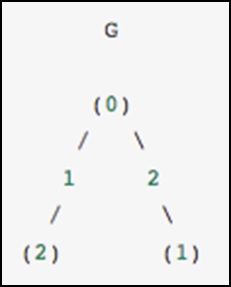
This graph has three nodes, where node 0 and 1 are connected by an edge of weight 2, and nodes 0 and 2 are connected by an edge of weight 1. We can construct the dense, masked and sparse representations as shown in the following example, keeping in mind that an undirected graph is represented by a symmetric matrix.
G_dense = np.array([ [0, 2, 1],
                     [2, 0, 0],
                     [1, 0, 0] ])

G_masked = np.ma.masked_values(G_dense, 0)
from scipy.sparse import csr_matrix

G_sparse = csr_matrix(G_dense)
print G_sparse.data
The above program will generate the following output.
array([2, 1, 2, 1])
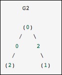
This is identical to the previous graph, except nodes 0 and 2 are connected by an edge of zero weight. In this case, the dense representation above leads to ambiguities − how can non-edges be represented, if zero is a meaningful value. In this case, either a masked or a sparse representation must be used to eliminate the ambiguity.
Let us consider the following example.
from scipy.sparse.csgraph import csgraph_from_dense
G2_data = np.array
([
   [np.inf, 2, 0 ],
   [2, np.inf, np.inf],
   [0, np.inf, np.inf]
])
G2_sparse = csgraph_from_dense(G2_data, null_value=np.inf)
print G2_sparse.data
The above program will generate the following output.
array([ 2., 0., 2., 0.])
Word ladders using sparse graphs
Word ladders is a game invented by Lewis Carroll, in which words are linked by changing a single letter at each step. For example −
APE → APT → AIT → BIT → BIG → BAG → MAG → MAN
Here, we have gone from "APE" to "MAN" in seven steps, changing one letter each time. The question is - Can we find a shorter path between these words using the same rule? This problem is naturally expressed as a sparse graph problem. The nodes will correspond to individual words, and we will create connections between words that differ by at the most one letter.
Obtaining a List of Words
First, of course, we must obtain a list of valid words. I am running Mac, and Mac has a word dictionary at the location given in the following code block. If you are on a different architecture, you may have to search a bit to find your system dictionary.
wordlist = open('/usr/share/dict/words').read().split()
print len(wordlist)
The above program will generate the following output.
235886
We now want to look at words of length 3, so let us select just those words of the correct length. We will also eliminate words, which start with upper case (proper nouns) or contain non-alpha-numeric characters such as apostrophes and hyphens. Finally, we will make sure everything is in lower case for a comparison later on.
word_list = [word for word in word_list if len(word) == 3]
word_list = [word for word in word_list if word[0].islower()]
word_list = [word for word in word_list if word.isalpha()]
word_list = map(str.lower, word_list)
print len(word_list)
The above program will generate the following output.
1135
Now, we have a list of 1135 valid three-letter words (the exact number may change depending on the particular list used). Each of these words will become a node in our graph, and we will create edges connecting the nodes associated with each pair of words, which differs by only one letter.
import numpy as np
word_list = np.asarray(word_list)

word_list.dtype
word_list.sort()

word_bytes = np.ndarray((word_list.size, word_list.itemsize),
   dtype = 'int8',
   buffer = word_list.data)
print word_bytes.shape
The above program will generate the following output.
(1135, 3)
We will use the Hamming distance between each point to determine, which pairs of words are connected. The Hamming distance measures the fraction of entries between two vectors, which differ: any two words with a hamming distance equal to 1/N1/N, where NN is the number of letters, which are connected in the word ladder.
from scipy.spatial.distance import pdist, squareform
from scipy.sparse import csr_matrix
hamming_dist = pdist(word_bytes, metric = 'hamming')
graph = csr_matrix(squareform(hamming_dist < 1.5 / word_list.itemsize))
When comparing the distances, we do not use equality because this can be unstable for floating point values. The inequality produces the desired result as long as no two entries of the word list are identical. Now, that our graph is set up, we will use the shortest path search to find the path between any two words in the graph.
i1 = word_list.searchsorted('ape')
i2 = word_list.searchsorted('man')
print word_list[i1],word_list[i2]
The above program will generate the following output.
ape, man
We need to check that these match, because if the words are not in the list there will be an error in the output. Now, all we need is to find the shortest path between these two indices in the graph. We will use dijkstras algorithm, because it allows us to find the path for just one node.
from scipy.sparse.csgraph import dijkstra
distances, predecessors = dijkstra(graph, indices = i1, return_predecessors = True)
print distances[i2]
The above program will generate the following output.
5.0
Thus, we see that the shortest path between ape and man contains only five steps. We can use the predecessors returned by the algorithm to reconstruct this path.
path = []
i = i2

while i != i1:
   path.append(word_list[i])
   i = predecessors[i]

path.append(word_list[i1])
print path[::-1]i2]
The above program will generate the following output.
['ape', 'ope', 'opt', 'oat', 'mat', 'man']
SciPy - Spatial
The scipy.spatial package can compute Triangulations, Voronoi Diagrams and Convex Hulls of a set of points, by leveraging the Qhull library. Moreover, it contains KDTree implementations for nearest-neighbor point queries and utilities for distance computations in various metrics.
Delaunay Triangulations
Let us understand what Delaunay Triangulations are and how they are used in SciPy.
What are Delaunay Triangulations?
In mathematics and computational geometry, a Delaunay triangulation for a given set P of discrete points in a plane is a triangulation DT(P) such that no point in P is inside the circumcircle of any triangle in DT(P).
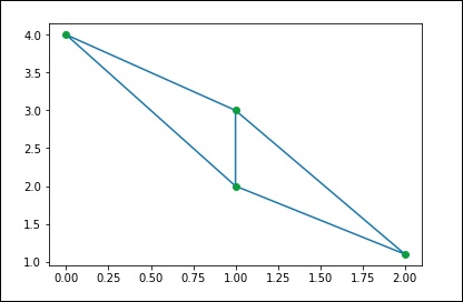
We can the compute the same through SciPy. Let us consider the following example.
from scipy.spatial import Delaunay
points = np.array([[0, 4], [2, 1.1], [1, 3], [1, 2]])
tri = Delaunay(points)
import matplotlib.pyplot as plt
plt.triplot(points[:,0], points[:,1], tri.simplices.copy())
plt.plot(points[:,0], points[:,1], 'o')
plt.show()
The above program will generate the following output.
Coplanar Points
Let us understand what Coplanar Points are and how they are used in SciPy.
What are Coplanar Points?
Coplanar points are three or more points that lie in the same plane. Recall that a plane is a flat surface, which extends without end in all directions. It is usually shown in math textbooks as a four-sided figure.
Let us see how we can find this using SciPy. Let us consider the following example.
from scipy.spatial import Delaunay
points = np.array([[0, 0], [0, 1], [1, 0], [1, 1], [1, 1]])
tri = Delaunay(points)
print tri.coplanar
The above program will generate the following output.
array([[4, 0, 3]], dtype = int32)
This means that point 4 resides near triangle 0 and vertex 3, but is not included in the triangulation.
Convex hulls
Let us understand what convex hulls are and how they are used in SciPy.
What are Convex Hulls?
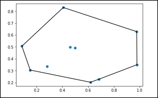
In mathematics, the convex hull or convex envelope of a set of points X in the Euclidean plane or in a Euclidean space (or, more generally, in an affine space over the reals) is the smallest convex set that contains X.
Let us consider the following example to understand it in detail.
from scipy.spatial import ConvexHull
points = np.random.rand(10, 2) # 30 random points in 2-D
hull = ConvexHull(points)
import matplotlib.pyplot as plt
plt.plot(points[:,0], points[:,1], 'o')
for simplex in hull.simplices:
plt.plot(points[simplex,0], points[simplex,1], 'k-')
plt.show()
The above program will generate the following output.
SciPy - ODR
ODR stands for Orthogonal Distance Regression, which is used in the regression studies. Basic linear regression is often used to estimate the relationship between the two variables y and x by drawing the line of best fit on the graph.
The mathematical method that is used for this is known as Least Squares, and aims to minimize the sum of the squared error for each point. The key question here is how do you calculate the error (also known as the residual) for each point?
In a standard linear regression, the aim is to predict the Y value from the X value so the sensible thing to do is to calculate the error in the Y values (shown as the gray lines in the following image). However, sometimes it is more sensible to take into account the error in both X and Y (as shown by the dotted red lines in the following image).
For example − When you know your measurements of X are uncertain, or when you do not want to focus on the errors of one variable over another.
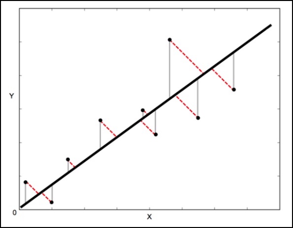
Orthogonal Distance Regression (ODR) is a method that can do this (orthogonal in this context means perpendicular so it calculates errors perpendicular to the line, rather than just vertically).
scipy.odr Implementation for Univariate Regression
The following example demonstrates scipy.odr implementation for univariate regression.
import numpy as np
import matplotlib.pyplot as plt
from scipy.odr import *
import random

# Initiate some data, giving some randomness using random.random().
x = np.array([0, 1, 2, 3, 4, 5])
y = np.array([i**2 + random.random() for i in x])

# Define a function (quadratic in our case) to fit the data with.
def linear_func(p, x):
   m, c = p
   return m*x + c

# Create a model for fitting.
linear_model = Model(linear_func)

# Create a RealData object using our initiated data from above.
data = RealData(x, y)

# Set up ODR with the model and data.
odr = ODR(data, linear_model, beta0=[0., 1.])

# Run the regression.
out = odr.run()

# Use the in-built pprint method to give us results.
out.pprint()
The above program will generate the following output.
Beta: [ 5.51846098 -4.25744878]
Beta Std Error: [ 0.7786442 2.33126407]

Beta Covariance: [
   [ 1.93150969 -4.82877433]
   [ -4.82877433 17.31417201
]]

Residual Variance: 0.313892697582
Inverse Condition #: 0.146618499389
Reason(s) for Halting:
   Sum of squares convergence
SciPy - Special Package
The functions available in the special package are universal functions, which follow broadcasting and automatic array looping.
Let us look at some of the most frequently used special functions −
- Cubic Root Function
- Exponential Function
- Relative Error Exponential Function
- Log Sum Exponential Function
- Lambert Function
- Permutations and Combinations Function
- Gamma Function
Let us now understand each of these functions in brief.
Cubic Root Function
The syntax of this cubic root function is scipy.special.cbrt(x). This will fetch the element-wise cube root of x.
Let us consider the following example.
from scipy.special import cbrt
res = cbrt([10, 9, 0.1254, 234])
print res
The above program will generate the following output.
[ 2.15443469 2.08008382 0.50053277 6.16224015]
Exponential Function
The syntax of the exponential function is scipy.special.exp10(x). This will compute 10**x element wise.
Let us consider the following example.
from scipy.special import exp10
res = exp10([2, 9])
print res
The above program will generate the following output.
[1.00000000e+02 1.00000000e+09]
Relative Error Exponential Function
The syntax for this function is scipy.special.exprel(x). It generates the relative error exponential, (exp(x) - 1)/x.
When x is near zero, exp(x) is near 1, so the numerical calculation of exp(x) - 1 can suffer from catastrophic loss of precision. Then exprel(x) is implemented to avoid the loss of precision, which occurs when x is near zero.
Let us consider the following example.
from scipy.special import exprel
res = exprel([-0.25, -0.1, 0, 0.1, 0.25])
print res
The above program will generate the following output.
[0.88479687 0.95162582 1. 1.05170918 1.13610167]
Log Sum Exponential Function
The syntax for this function is scipy.special.logsumexp(x). It helps to compute the log of the sum of exponentials of input elements.
Let us consider the following example.
from scipy.special import logsumexp
import numpy as np
a = np.arange(10)
res = logsumexp(a)
print res
The above program will generate the following output.
9.45862974443
Lambert Function
The syntax for this function is scipy.special.lambertw(x). It is also called as the Lambert W function. The Lambert W function W(z) is defined as the inverse function of w * exp(w). In other words, the value of W(z) is such that z = W(z) * exp(W(z)) for any complex number z.
The Lambert W function is a multivalued function with infinitely many branches. Each branch gives a separate solution of the equation z = w exp(w). Here, the branches are indexed by the integer k.
Let us consider the following example. Here, the Lambert W function is the inverse of w exp(w).
from scipy.special import lambertw
w = lambertw(1)
print w
print w * np.exp(w)
The above program will generate the following output.
(0.56714329041+0j)
(1+0j)
Permutations & Combinations
Let us discuss permutations and combinations separately for understanding them clearly.
Combinations − The syntax for combinations function is scipy.special.comb(N,k). Let us consider the following example −
from scipy.special import comb
res = comb(10, 3, exact = False,repetition=True)
print res
The above program will generate the following output.
220.0
Note − Array arguments are accepted only for exact = False case. If k > N, N < 0, or k < 0, then a 0 is returned.
Permutations − The syntax for combinations function is scipy.special.perm(N,k). Permutations of N things taken k at a time, i.e., k-permutations of N. This is also known as partial permutations.
Let us consider the following example.
from scipy.special import perm
res = perm(10, 3, exact = True)
print res
The above program will generate the following output.
720
Gamma Function
The gamma function is often referred to as the generalized factorial since z*gamma(z) = gamma(z+1) and gamma(n+1) = n!, for a natural number n.
The syntax for combinations function is scipy.special.gamma(x). Permutations of N things taken k at a time, i.e., k-permutations of N. This is also known as partial permutations.
The syntax for combinations function is scipy.special.gamma(x). Permutations of N things taken k at a time, i.e., k-permutations of N. This is also known as partial permutations.
from scipy.special import gamma
res = gamma([0, 0.5, 1, 5])
print res
The above program will generate the following output.
[inf 1.77245385 1. 24.]
