- SciPy - Home
- SciPy - Introduction
- SciPy - Environment Setup
- SciPy - Basic Functionality
- SciPy - Relationship with NumPy
- SciPy Clusters
- SciPy - Clusters
- SciPy - Hierarchical Clustering
- SciPy - K-means Clustering
- SciPy - Distance Metrics
- SciPy Constants
- SciPy - Constants
- SciPy - Mathematical Constants
- SciPy - Physical Constants
- SciPy - Unit Conversion
- SciPy - Astronomical Constants
- SciPy - Fourier Transforms
- SciPy - FFTpack
- SciPy - Discrete Fourier Transform (DFT)
- SciPy - Fast Fourier Transform (FFT)
- SciPy Integration Equations
- SciPy - Integrate Module
- SciPy - Single Integration
- SciPy - Double Integration
- SciPy - Triple Integration
- SciPy - Multiple Integration
- SciPy Differential Equations
- SciPy - Differential Equations
- SciPy - Integration of Stochastic Differential Equations
- SciPy - Integration of Ordinary Differential Equations
- SciPy - Discontinuous Functions
- SciPy - Oscillatory Functions
- SciPy - Partial Differential Equations
- SciPy Interpolation
- SciPy - Interpolate
- SciPy - Linear 1-D Interpolation
- SciPy - Polynomial 1-D Interpolation
- SciPy - Spline 1-D Interpolation
- SciPy - Grid Data Multi-Dimensional Interpolation
- SciPy - RBF Multi-Dimensional Interpolation
- SciPy - Polynomial & Spline Interpolation
- SciPy Curve Fitting
- SciPy - Curve Fitting
- SciPy - Linear Curve Fitting
- SciPy - Non-Linear Curve Fitting
- SciPy - Input & Output
- SciPy - Input & Output
- SciPy - Reading & Writing Files
- SciPy - Working with Different File Formats
- SciPy - Efficient Data Storage with HDF5
- SciPy - Data Serialization
- SciPy Linear Algebra
- SciPy - Linalg
- SciPy - Matrix Creation & Basic Operations
- SciPy - Matrix LU Decomposition
- SciPy - Matrix QU Decomposition
- SciPy - Singular Value Decomposition
- SciPy - Cholesky Decomposition
- SciPy - Solving Linear Systems
- SciPy - Eigenvalues & Eigenvectors
- SciPy Image Processing
- SciPy - Ndimage
- SciPy - Reading & Writing Images
- SciPy - Image Transformation
- SciPy - Filtering & Edge Detection
- SciPy - Top Hat Filters
- SciPy - Morphological Filters
- SciPy - Low Pass Filters
- SciPy - High Pass Filters
- SciPy - Bilateral Filter
- SciPy - Median Filter
- SciPy - Non - Linear Filters in Image Processing
- SciPy - High Boost Filter
- SciPy - Laplacian Filter
- SciPy - Morphological Operations
- SciPy - Image Segmentation
- SciPy - Thresholding in Image Segmentation
- SciPy - Region-Based Segmentation
- SciPy - Connected Component Labeling
- SciPy Optimize
- SciPy - Optimize
- SciPy - Special Matrices & Functions
- SciPy - Unconstrained Optimization
- SciPy - Constrained Optimization
- SciPy - Matrix Norms
- SciPy - Sparse Matrix
- SciPy - Frobenius Norm
- SciPy - Spectral Norm
- SciPy Condition Numbers
- SciPy - Condition Numbers
- SciPy - Linear Least Squares
- SciPy - Non-Linear Least Squares
- SciPy - Finding Roots of Scalar Functions
- SciPy - Finding Roots of Multivariate Functions
- SciPy - Signal Processing
- SciPy - Signal Filtering & Smoothing
- SciPy - Short-Time Fourier Transform
- SciPy - Wavelet Transform
- SciPy - Continuous Wavelet Transform
- SciPy - Discrete Wavelet Transform
- SciPy - Wavelet Packet Transform
- SciPy - Multi-Resolution Analysis
- SciPy - Stationary Wavelet Transform
- SciPy - Statistical Functions
- SciPy - Stats
- SciPy - Descriptive Statistics
- SciPy - Continuous Probability Distributions
- SciPy - Discrete Probability Distributions
- SciPy - Statistical Tests & Inference
- SciPy - Generating Random Samples
- SciPy - Kaplan-Meier Estimator Survival Analysis
- SciPy - Cox Proportional Hazards Model Survival Analysis
- SciPy Spatial Data
- SciPy - Spatial
- SciPy - Special Functions
- SciPy - Special Package
- SciPy Advanced Topics
- SciPy - CSGraph
- SciPy - ODR
- SciPy Useful Resources
- SciPy - Reference
- SciPy - Quick Guide
- SciPy - Cheatsheet
- SciPy - Useful Resources
- SciPy - Discussion
SciPy - ODR
ODR stands for Orthogonal Distance Regression, which is used in the regression studies. Basic linear regression is often used to estimate the relationship between the two variables y and x by drawing the line of best fit on the graph.
The mathematical method that is used for this is known as Least Squares, and aims to minimize the sum of the squared error for each point. The key question here is how do you calculate the error (also known as the residual) for each point?
In a standard linear regression, the aim is to predict the Y value from the X value so the sensible thing to do is to calculate the error in the Y values (shown as the gray lines in the following image). However, sometimes it is more sensible to take into account the error in both X and Y (as shown by the dotted red lines in the following image).
For example − When you know your measurements of X are uncertain, or when you do not want to focus on the errors of one variable over another.
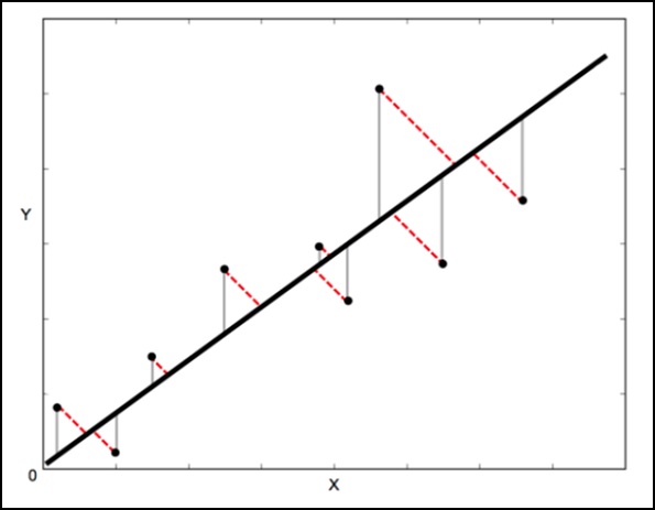
Orthogonal Distance Regression (ODR) is a method that can do this (orthogonal in this context means perpendicular so it calculates errors perpendicular to the line, rather than just vertically).
scipy.odr Implementation for Univariate Regression
The following example demonstrates scipy.odr implementation for univariate regression.
import numpy as np
import matplotlib.pyplot as plt
from scipy.odr import *
import random

# Initiate some data, giving some randomness using random.random().
x = np.array([0, 1, 2, 3, 4, 5])
y = np.array([i**2 + random.random() for i in x])

# Define a function (quadratic in our case) to fit the data with.
def linear_func(p, x):
   m, c = p
   return m*x + c

# Create a model for fitting.
linear_model = Model(linear_func)

# Create a RealData object using our initiated data from above.
data = RealData(x, y)

# Set up ODR with the model and data.
odr = ODR(data, linear_model, beta0=[0., 1.])

# Run the regression.
out = odr.run()

# Use the in-built pprint method to give us results.
out.pprint()
Output
The above program will generate the following output.
Beta: [ 5.51846098 -4.25744878]
Beta Std Error: [ 0.7786442 2.33126407]

Beta Covariance: [
   [ 1.93150969 -4.82877433]
   [ -4.82877433 17.31417201
]]

Residual Variance: 0.313892697582
Inverse Condition #: 0.146618499389
Reason(s) for Halting:
   Sum of squares convergence
