SciPy - Polynomial & Spline Interpolation

---

---

Interpolation is a method of estimating unknown values that fall within the range of a discrete set of known data points. SciPy provides various tools for polynomial and spline interpolation which allows for flexible modeling of data.

Polynomial Interpolation

Polynomial interpolation is a process of estimating values between known data points by fitting a polynomial to a set of points. Then n+1 data points are given as (x₀,y₀), (x₁,y₁).......,(x_n,y_n) then the goal is to find a polynomial P(x) of degree n which is given as follows −

P(xi) = yi for all i = 0,1,....,n

General Form of Polynomial Interpolation

The interpolating polynomial can be written in general as follows −

P(x) = a0+a1x+a2x2+......+anxn

Where, a₀, a₁,......,a_n are the coefficients that we need to determine.

Methods of Polynomial Interpolation

Polynomial interpolation involves fitting a polynomial function that passes through a given set of data points. There are various methods to construct such a polynomial. Here are the most common methods of polynomial interpolation −

Lagrange Interpolation

Lagrange interpolation constructs the polynomial by combining Lagrange basis polynomials with each corresponding to a data point. This method does not require solving a system of equations.

The Lagrange interpolation Polynomial P(x) for n+1 data points (x₀,y₀), (x₁,y₁).......,(x_n,y_n) is given as follows −

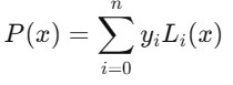
Where, L_i(x) are the Lagrange basis polynomials defined as −

Following are the characteristics of the Lagrange Polynomial Interpolation in Scipy −

• No need to solve a linear system.

• Efficient for small datasets but becomes inefficient for large datasets.

• Suffer from Runges phenomenon (oscillations) with large datasets.

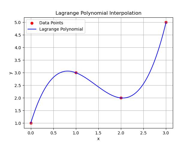
Example

Heres an example of Lagrange polynomial interpolation using the scipy.interpolate.lagrange() function. This method constructs the Lagrange polynomial that passes through a given set of data points −

import numpy as np
import matplotlib.pyplot as plt
from scipy.interpolate import lagrange

# Define the data points (x, y)
x = np.array([0, 1, 2, 3])
y = np.array([1, 3, 2, 5])

# Construct the Lagrange polynomial using scipy
polynomial = lagrange(x, y)

# Generate points to plot the interpolated polynomial
x_new = np.linspace(0, 3, 100)
y_new = polynomial(x_new)

# Plot the data points and the Lagrange polynomial
plt.scatter(x, y, color='red', label='Data Points')
plt.plot(x_new, y_new, label='Lagrange Polynomial', color='blue')

# Add labels and title
plt.title('Lagrange Polynomial Interpolation')
plt.xlabel('x')
plt.ylabel('y')
plt.legend()
plt.grid(True)
plt.show()

# Print the polynomial for reference
print(f"Lagrange Polynomial:\n{polynomial}")

Output

Following is the output of the Lagrange Polynomial Interpolation −

Lagrange Polynomial:
       3     2
1.167 x - 5 x + 5.833 x + 1

Newton's Interpolation

Newtons interpolation is based on constructing the polynomial using divided differences. It is more efficient than Lagrange for adding new data points.

The Newton form of the interpolating polynomial is is given as follows −

P(x) = f[x0]+f[x0,x1](x-x0)+f[x0,x1,x2](x-x0)(x-x1).....f[x0,x1,....,xn](x-x0)(x-x1)....(x-xn)

Where, f[x₀,x₁,....,x_n] are the divided differences computed iteratively from the data points.

Below are the characteristics of Newton's Interpolation in scipy −

• Efficient for incremental data points.

• Easier to update when adding more data.

• Less prone to oscillation compared to Lagrange interpolation.

Example

In SciPy there is no direct function for Newton's divided difference interpolation like there is for Lagrange Interpolation. However we can implement Newton's interpolation using the divided differences formula manually. Here's an example of how to perform Newton's interpolation in Python using SciPy for basic operations −

import numpy as np
import matplotlib.pyplot as plt

# Function to calculate divided differences
def divided_diff(x, y):
    n = len(y)
    coef = np.zeros([n, n])
    coef[:, 0] = y  # First column is y

    for j in range(1, n):
        for i in range(n - j):
            coef[i, j] = (coef[i + 1, j - 1] - coef[i, j - 1]) / (x[i + j] - x[i])
    
    return coef[0, :]  # Return the first row (Newton's coefficients)

# Function to evaluate Newton's polynomial at a given x
def newton_polynomial(coef, x_data, x):
    n = len(coef) - 1
    p = coef[n]
    for k in range(1, n + 1):
        p = coef[n - k] + (x - x_data[n - k]) * p
    return p

# Define data points (x, y)
x = np.array([1, 2, 3, 4])
y = np.array([1, 4, 9, 16])  # y = x^2 for example

# Compute divided differences coefficients
coefficients = divided_diff(x, y)

# Generate points for plotting
x_new = np.linspace(1, 4, 100)
y_new = [newton_polynomial(coefficients, x, xi) for xi in x_new]

# Plot the original points and the Newton interpolating polynomial
plt.scatter(x, y, color='red', label='Data Points')
plt.plot(x_new, y_new, label='Newton Polynomial', color='blue')

# Add labels and title
plt.title("Newton's Divided Difference Interpolation")
plt.xlabel('x')
plt.ylabel('y')
plt.legend()
plt.grid(True)
plt.show()

# Print the divided difference coefficients
print(f"Newton's Divided Difference Coefficients: {coefficients}")

Output

Following is the output of the Newton's divided difference Polynomial Interpolation −

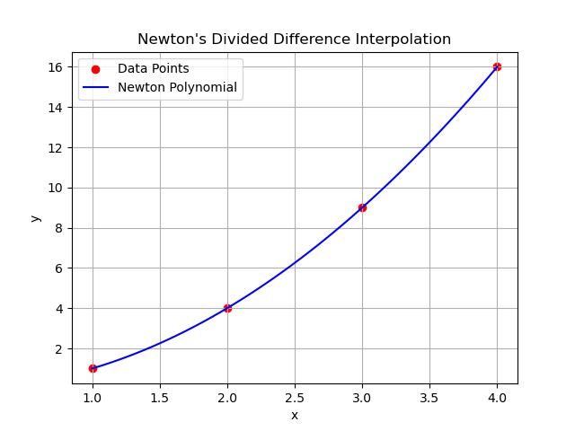
Newton's Divided Difference Coefficients: [1. 3. 1. 0.]

Vandermonde Matrix Method

The Vandermonde matrix method constructs a system of linear equations based on the data points. Solving the system provides the polynomial coefficients.

For n+1 points (x₀,y₀), (x₁,y₁).......,(x_n,y_n), the polynomial a₀+a₁x+a₂x²+......+a_nxⁿ can be written as a system of linear equations −

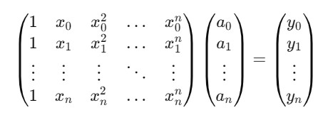
This is the Vandermonde matrix () and solving the linear system (). = gives the coefficients _i.

The characteristics of Vandermonde matrix are given as follows −

• Direct and simple approach for small datasets.

• Computationally expensive and numerically unstable for large datasets due to the ill-conditioning of the Vandermonde matrix.

Example

Here's an example of how to use the Vandermonde matrix method to perform polynomial interpolation in Python. This method constructs a system of linear equations to solve for the polynomial coefficients that pass through a given set of data points −

import numpy as np
import matplotlib.pyplot as plt

# Define the data points (x, y)
x = np.array([0, 1, 2, 3])
y = np.array([1, 3, 2, 5])

# Construct the Vandermonde matrix
V = np.vander(x, increasing=True)

# Solve for the polynomial coefficients
coefficients = np.linalg.solve(V, y)

# Define a function to represent the interpolated polynomial
def polynomial_function(x_val):
    return sum(c * (x_val ** i) for i, c in enumerate(coefficients))

# Generate points for plotting the interpolated polynomial
x_new = np.linspace(0, 3, 100)
y_new = polynomial_function(x_new)

# Plot the original data points and the polynomial interpolation
plt.scatter(x, y, color='red', label='Data Points')
plt.plot(x_new, y_new, label='Vandermonde Polynomial', color='blue')

# Add labels and title
plt.title('Vandermonde Matrix Polynomial Interpolation')
plt.xlabel('x')
plt.ylabel('y')
plt.legend()
plt.grid(True)
plt.show()

# Print the polynomial coefficients for reference
print(f"Polynomial Coefficients: {coefficients}")

Output

Following is the output of the Vandermonde Matrix Interpolation −

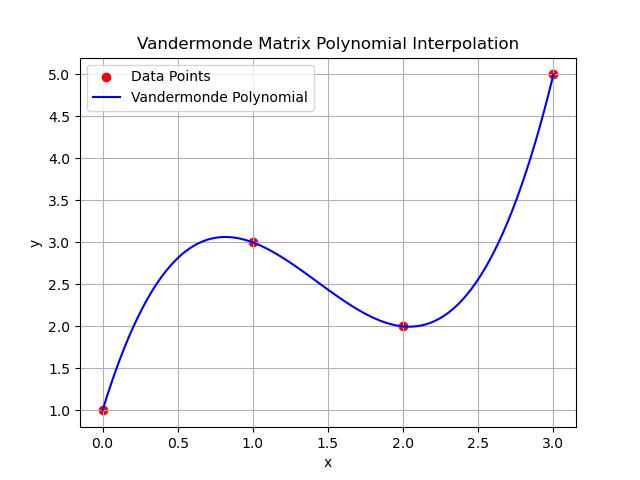
Polynomial Coefficients: [ 1.          5.83333333 -5.          1.16666667]

Hermite Interpolation

Hermite interpolation not only matches the function values at given data points but also ensures that the derivatives i.e., slopes match if known. It is an extension of polynomial interpolation when derivative information is available.

For a dataset (x₀,f(x₀),f(x₀)),(x₁,f(x₁),f(x₁)),......,(x_n,f(x_n),f(x_n)), the Hermite polynomial H(x)is constructed using divided differences similar to Newtons interpolation but including derivative information.

Here are the characteristics of Hermite Interpolationof Scipy −

• Ensures smooth transitions between points by matching slopes.

• Suitable when derivative information is available or needed.

• More complex to compute than standard polynomial interpolation.

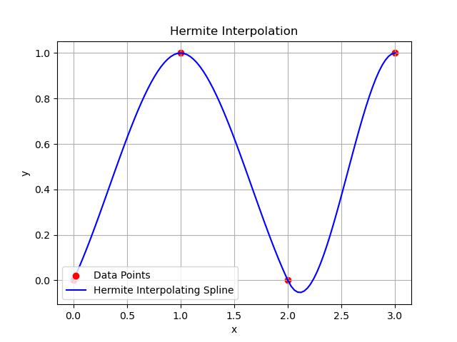
Example

Heres an example of Hermite interpolation using scipy.interpolate.BarycentricInterpolator() function for polynomial interpolation. For true Hermite interpolation i.e., interpolating both function values and derivatives we can use scipy.interpolate.CubicHermiteSpline() function −

import numpy as np
import matplotlib.pyplot as plt
from scipy.interpolate import CubicHermiteSpline

# Define the data points (x, y) and the derivative values (dy)
x = np.array([0, 1, 2, 3])
y = np.array([0, 1, 0, 1])   # Function values at the data points
dy = np.array([1, 0, -1, 0])  # Derivatives at the data points

# Construct the Hermite cubic spline
hermite_spline = CubicHermiteSpline(x, y, dy)

# Generate points for plotting the interpolated curve
x_new = np.linspace(0, 3, 100)
y_new = hermite_spline(x_new)

# Plot the data points and Hermite interpolating spline
plt.scatter(x, y, color='red', label='Data Points')
plt.plot(x_new, y_new, label='Hermite Interpolating Spline', color='blue')

# Add labels and title
plt.title('Hermite Interpolation')
plt.xlabel('x')
plt.ylabel('y')
plt.legend()
plt.grid(True)
plt.show()

Output

Here is the output of the Hermite Interpolation −

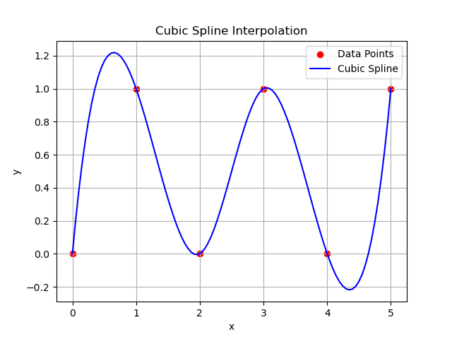
Spline Interpolation

Spline interpolation in SciPy involves fitting piecewise polynomials i.e., usually cubic polynomials between data points to create a smooth curve. The most commonly used spline in SciPy is the cubic spline which ensures that the curve is smooth and continuous at the data points and minimizes oscillations that occur in higher-degree polynomial interpolation.

The Spline Interpolation is of two types namely Cubic spline which ensures that the curve is continuous and has continuous first and second derivatives at the data points and the Natural Spline which is a cubic spline that has a second derivative of zero at the endpoints by providing a natural boundary condition.

Spline interpolation is widely used due to its smoothness and flexibility in Computer graphics and animation, Data smoothing and fitting and Robotics for trajectory planning.

Example

Following is the example which shows how to use the function scipy.interpolate.CubicHermiteSpline() for creating the Spline Interpolation in scipy −

import numpy as np
import matplotlib.pyplot as plt
from scipy.interpolate import CubicSpline

# Define the data points (x, y)
x = np.array([0, 1, 2, 3, 4, 5])
y = np.array([0, 1, 0, 1, 0, 1])

# Create the cubic spline interpolator
cubic_spline = CubicSpline(x, y)

# Generate points for plotting the interpolated curve
x_new = np.linspace(0, 5, 100)
y_new = cubic_spline(x_new)

# Plot the data points and the cubic spline
plt.scatter(x, y, color='red', label='Data Points')
plt.plot(x_new, y_new, label='Cubic Spline', color='blue')

# Add labels and title
plt.title('Cubic Spline Interpolation')
plt.xlabel('x')
plt.ylabel('y')
plt.legend()
plt.grid(True)
plt.show()

Output

Here is the output of the Spline Interpolation in scipy −