SciPy - ndimage.guassian_filter() Function

The scipy.ndimage.guassian_filter() is a function in the SciPy library which is used to apply a Gaussian filter to an input array i.e., typically an image or multidimensional data. It smooths the data by convolving it with a Gaussian kernel which has the effect of reducing noise and blurring the image.

This function allows to control over the standard deviation (sigma) of the Gaussian kernel in each dimension by affecting the extent of smoothing. It also accepts other parameters such as the size of the filter and the mode of boundary handling. It's commonly used for tasks like noise reduction and image pre-processing.

Syntax

Following is the syntax of the function scipy.ndimage.guassian_filter() to apply the Guassian Filter −

scipy.ndimage.gaussian_filter(input, sigma, order=0, mode='reflect', cval=0.0, truncate=4.0)

Parameters

Below are the parameters of the scipy.ndimage.guassian_filter() function −

• input (array_like): The input array (image or data) that will be processed.
• sigma (float or sequence of floats): The standard deviation of the Gaussian filter. If sigma is a single float then it applies the same value to all dimensions. If a sequence is provided then it must match the dimensions of the input array.
• footprint (array_like, optional): A boolean array that defines the shape of the neighborhood. This can be used instead of size. The default value is None.
• order (int or tuple of ints, optional): The order of the filter. It can be 0 ie., Gaussian filter or we can set it to higher values to apply derivatives of the Gaussian. Default value is 0.
• mode (str, optional): This parameter specifies how the input is extended when the filter overlaps with the boundary. The available modes in this filter are as follows −
  • reflect: This is the default value where the array is reflected at the boundaries.
  • constant: Pads with a constant value (specified by cval).
  • nearest: Pads with the nearest boundary value.
  • mirror: Similar to reflect but without copying the boundary values.
  • wrap: Wraps the array from the opposite side.
• cval (scalar, optional): This value is used for points outside the boundaries when mode='constant' and the default value is 0.0.
• truncate (float, optional): This parameter truncates the filter at this many standard deviations from the center. Default value is 4.0 which means the filter will effectively be zero beyond 4 standard deviations.

Return Value

The scipy.ndimage.guassian_filter() function returns the filtered image or array which is with the same shape as input where the elements are smoothed based on the Gaussian kernel.

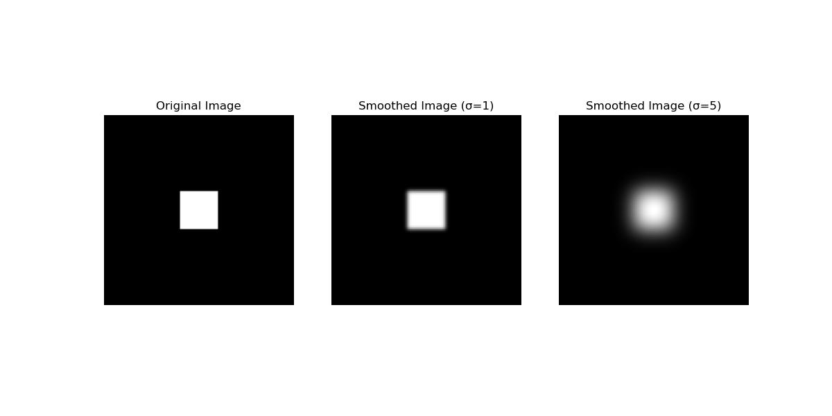
Basic Gaussian Blurring

Following is the basic example which uses scipy.ndimage.guassian_filter() function to perform simple Gaussian blurring applied to an image with varying levels of smoothing −

import numpy as np
import matplotlib.pyplot as plt
from scipy.ndimage import gaussian_filter

# Create a sample image (a 2D array with sharp edges)
image = np.zeros((100, 100))
image[40:60, 40:60] = 1  # Create a white square in the middle

# Apply Gaussian filter with different sigma values
smoothed_image_1 = gaussian_filter(image, sigma=1)  # Low smoothing
smoothed_image_2 = gaussian_filter(image, sigma=5)  # High smoothing

# Plot the original and smoothed images
plt.figure(figsize=(12, 6))

# Original image
plt.subplot(1, 3, 1)
plt.title("Original Image")
plt.imshow(image, cmap='gray')
plt.axis('off')

# Smoothed image with sigma=1
plt.subplot(1, 3, 2)
plt.title("Smoothed Image (=1)")
plt.imshow(smoothed_image_1, cmap='gray')
plt.axis('off')

# Smoothed image with sigma=5
plt.subplot(1, 3, 3)
plt.title("Smoothed Image (=5)")
plt.imshow(smoothed_image_2, cmap='gray')
plt.axis('off')

plt.show()

Here is the output of the basic Guassian filter which uses scipy.ndimage.guassian_filter() function −

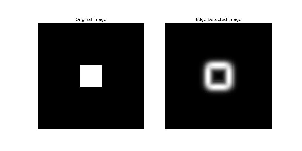
Gaussian Derivative (Edge Detection)

The Gaussian derivative is an essential tool in image processing which is particularly for edge detection. By using the Gaussian filter with a derivative operation i.e., first or higher-order where we can emphasize the edges in an image. This process detects rapid intensity changes and is often used in edge detection algorithms such as the Sobel filter or Canny edge detection.

Here is the example which shows how to perform edge detection using the first derivative of a Gaussian filter with scipy.ndimage.gaussian_filter() −

import numpy as np
import matplotlib.pyplot as plt
from scipy.ndimage import gaussian_filter

# Create a sample image (a 2D array with sharp edges)
image = np.zeros((100, 100))
image[40:60, 40:60] = 1  # Create a white square in the middle

# Derivative along the x-axis (horizontal)
edges_x = gaussian_filter(image, sigma=3, order=(1, 0))  # First derivative along x-axis

# Derivative along the y-axis (vertical)
edges_y = gaussian_filter(image, sigma=3, order=(0, 1))  # First derivative along y-axis

# Combine the x and y gradients to get the magnitude of edges
edges_magnitude = np.sqrt(edges_x**2 + edges_y**2)

# Plot the original and edge-detected images
plt.figure(figsize=(12, 6))

# Original image
plt.subplot(1, 2, 1)
plt.title("Original Image")
plt.imshow(image, cmap='gray')
plt.axis('off')

# Edge-detected image (gradient magnitude)
plt.subplot(1, 2, 2)
plt.title("Edge Detected Image")
plt.imshow(edges_magnitude, cmap='gray')
plt.axis('off')

plt.show()

Here is the output of the Guassian filter used to perform edge detection using scipy.ndimage.guassian_filter() function −

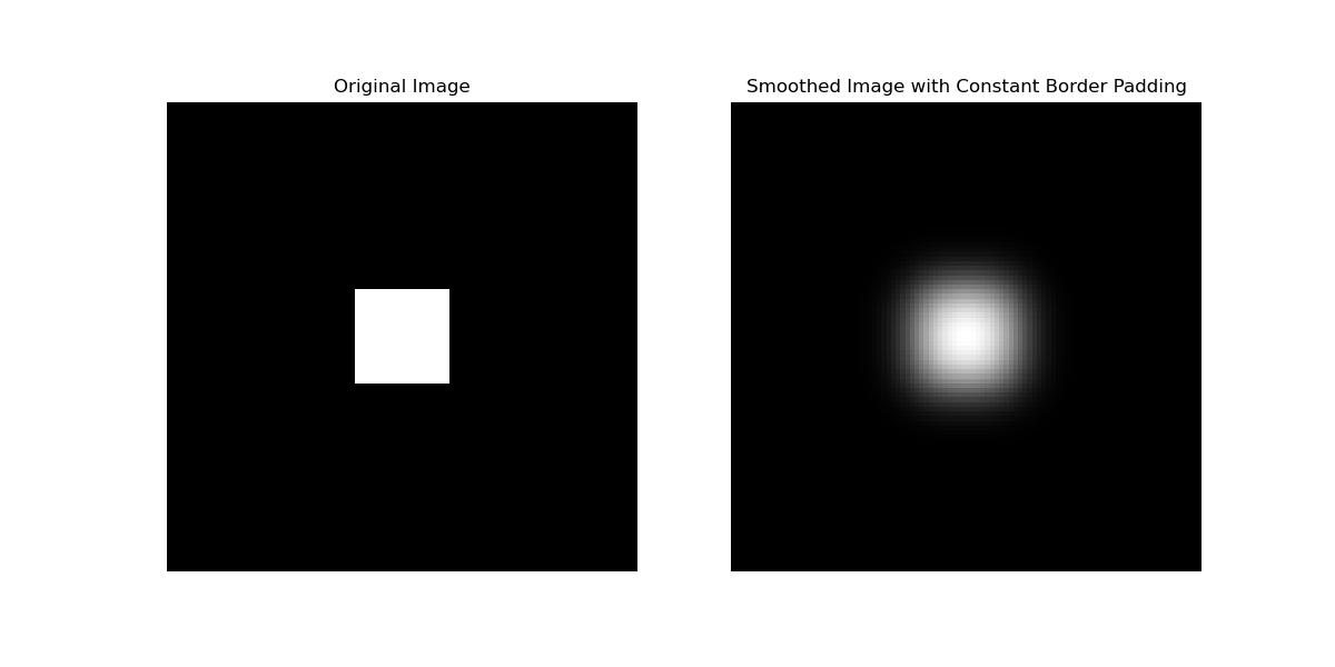
Gaussian Filter with Custom Border Handling

In this example we apply a Gaussian filter to an image with custom border handling using the mode and cval parameters of the scipy.ndimage.guassian_filter() function −

import numpy as np
import matplotlib.pyplot as plt
from scipy.ndimage import gaussian_filter

# Create a sample image with a sharp edge
image = np.zeros((100, 100))
image[40:60, 40:60] = 1  # Create a white square in the middle

# Apply Gaussian filter with 'constant' mode and custom constant value for padding
smoothed_image_constant = gaussian_filter(image, sigma=5, mode='constant', cval=0)

# Plot the original and smoothed images
plt.figure(figsize=(12, 6))

# Original image
plt.subplot(1, 2, 1)
plt.title("Original Image")
plt.imshow(image, cmap='gray')
plt.axis('off')

# Smoothed image with custom padding
plt.subplot(1, 2, 2)
plt.title("Smoothed Image with Constant Border Padding")
plt.imshow(smoothed_image_constant, cmap='gray')
plt.axis('off')

plt.show()

Here is the output of the Guassian filter used to perform custom border handling using scipy.ndimage.guassian_filter() function −